RMSTSS: Sample Size and Power Calculations for RMST-based Clinical Trials
Arnab Aich
RMSTSS.RmdIntroduction
The design and analysis of clinical trials with time-to-event endpoints often rely on the hazard-based model (e.g., the Cox model) and use the hazard ratio (HR) as the primary estimand of the treatment effect. However, the HR can be challenging to interpret from both clinical and causal perspectives. Moreover, the key assumption underlying most hazards models - the proportional hazards assumption - is often tenuous or violated in real-world settings.
As an alternative, the Restricted Mean Survival Time (RMST) is gaining favor for its straightforward interpretation and robust properties (Royston and Parmar 2013; Uno et al. 2014). The RMST measures the average event-free time up to a pre-specified follow-up point, . This provides a direct and meaningful measure of treatment benefit (e.g., “an average of 3 extra months of survival over 5 years”), which is highly valuable for clinicians and patients.
Modern statistical methods now focus on modeling the RMST directly as a function of baseline covariates, rather than estimating it indirectly from a survival curve or a hazard function. This direct approach, based on foundational work using Inverse Probability of Censoring Weighting (IPCW) (Tian, Zhao, and Wei 2014), has been extended to handle the complex data structures observed in modern trials, including facility profiling in multi-center studies or other stratification factors (Wang et al. 2019; Zhang and Schaubel 2024) and covariate-dependent censoring (Wang and Schaubel 2018).
However, most software tools for these advanced methods focus on analyzing existing data, not designing new studies. This has left trial statisticians to write custom code for the crucial task of calculating sample size and power.
The RMSTSS package is designed to fill this gap. It
provides a comprehensive and user-friendly suite of tools for
power and sample size calculations based on the latest
direct RMST methodologies. The package implements several key approaches
from the statistical literature:
- Generalized Linear Models: The foundational regression model for RMST with IPCW-based estimation (Tian, Zhao, and Wei 2014).
- Stratified Models: Efficient methods for studies with a large number of strata (e.g., clinical centers), including both additive (Zhang and Schaubel 2024) and multiplicative (Wang et al. 2019) models.
- Dependent Censoring Models: Methods for handling covariate-dependent censoring (Wang and Schaubel 2018).
- Flexible Non-Linear Models: Bootstrap-based functions using Generalized Additive Models (GAMs) to capture non-linear covariate effects.
-
Analytic vs. Bootstrap Methods: For most models,
the package offers a choice between a fast
analyticalcalculation and a robust, simulation-basedbootmethod.
This vignette will guide you through the theory and application of each of these function groups.
Core Concepts of RMSTSS Package
The RMSTSS package uses two primary approaches for its
calculations: a fast Analytic Method and a robust
Bootstrap Method. All functions for finding sample size
then use a common search algorithm. Understanding these three components
is key to choosing the right function for your needs.
The Analytic Method (.analytical functions)
The analytical functions are extremely fast because they use a direct mathematical formula to calculate power. This makes them ideal for quickly exploring different scenarios. The process is:
-
One-Time Estimation: The function first analyzes
the provided
pilot_datato estimate two key parameters:- The treatment effect size (e.g., the difference in RMST or the log-RMST ratio).
- The asymptotic variance of that effect estimator, which measures its uncertainty.
-
Power Formula: It then plugs these fixed estimates
into a standard power formula. For a given total sample size
N, the power is calculated as: where:- is the cumulative distribution function (CDF) of the standard normal distribution.
- is the treatment effect estimated from the pilot data.
-
is the standard error of the effect for the target sample size
N, which is scaled from the pilot data’s variance. - is the critical value from the standard normal distribution (e.g., 1.96 for an alpha of 0.05).
The Bootstrap Method (.boot functions)
The bootstrap functions provide a robust, simulation-based alternative that makes fewer assumptions about the data’s distribution. This is a trade-off, as they are much more computationally intensive. The process is:
-
Resample: The function simulates a “future trial”
of a given
sample_sizeby resampling with replacement from thepilot_data. - Fit Model: On this new bootstrap sample, it performs the full analysis (e.g., calculating weights or pseudo-observations and fitting the specified model).
- Get P-Value: It extracts the p-value for the treatment effect from the fitted model.
-
Repeat: This process is repeated thousands of times
(
n_sim). -
Calculate Power: The final estimated power is the
proportion of simulations where the p-value was less than the
significance level
alpha.
The Sample Size Search Algorithm (.ss functions)
All functions ending in .ss (for sample size) use the
same iterative search algorithm to find the N required to
achieve a target_power:
-
Start: The search begins with a sample size of
n_start. -
Calculate Power: It calculates the power for the
current_nusing either the analytic formula or a full bootstrap simulation. -
Check Condition:
- If
calculated_power >= target_power, the search succeeds and returnscurrent_n. - If not, it increments the sample size
(
current_n = current_n + n_step) and repeats the process.
- If
-
Stopping Rules: The search terminates if the sample
size exceeds
max_n_per_armor, for bootstrap methods, if the power fails to improve for a set number ofpatiencesteps.
Avaailable Functions: A Quick Guide
The package uses a consistent naming convention to help you select
the correct function. The names are combinations of the
[Model Type], the [Goal - power or ss], and
the [Method - analytical or boot]. The table below provides
a summary of the available functions for each model.
| Model Type | Analytic Functions | Bootstrap Functions |
|---|---|---|
| Linear IPCW |
linear.power.analytical
linear.ss.analytical
|
linear.power.boot
linear.ss.boot
|
| Additive Stratified |
additive.power.analytical
additive.ss.analytical
|
Not applicable |
| Multiplicative Stratified |
MS.power.analytical
MS.ss.analytical
|
MS.power.boot
MS.ss.boot
|
| Semiparametric GAM | Not applicable |
GAM.power.boot
GAM.ss.boot
|
| Dependent Censoring |
DC.power.analytical
DC.ss.analytical
|
Not applicable |
Selecting an Appropriate Model
Model selection depends on the assumptions made about the data structure and the design of the study. The following table summarizes recommended modeling strategies under various analytical scenarios:
| Model | Key Assumption / Scenario | Recommended Use Case |
|---|---|---|
| Linear IPCW | Assumes a linear relationship between covariates and RMST. | Suitable for baseline analyses where there is no strong evidence of non-linear effects or complex stratification. |
| Additive Stratified | Assumes the treatment adds a constant amount of survival time across strata. | Appropriate for multi-center trials where the treatment effect is expected to be uniform (e.g., a fixed increase in survival time across centers). |
| Multiplicative Stratified | Assumes the treatment multiplies survival time proportionally across strata. | Preferred in multi-center trials where the treatment is expected to produce proportional gains relative to baseline survival across different centers. |
| Semiparametric GAM | Allows for non-linear covariate effects on RMST. | Useful when variables (e.g., age, biomarker levels) are believed to have complex, non-linear associations with the outcome. |
| Dependent Censoring | Accounts for dependent censoring or competing risks. | Recommended for studies involving competing events, such as transplant studies where receiving a transplant precludes observation of pre-transplant mortality. |
Linear IPCW Models
These functions implement the foundational direct linear regression model for the RMST. This model is appropriate when a linear relationship between covariates and the RMST is assumed, and when censoring is independent of the event of interest.
Theory and Model
Based on the methods of (Tian, Zhao, and Wei 2014), these functions model the conditional RMST as a linear function of covariates: In this model, the expected RMST up to a pre-specified time L for subject i is modeled as a linear combination of their treatment arm and other variables .
To handle right-censoring, the method uses Inverse Probability of Censoring Weighting (IPCW). This is achieved through the following steps:
- A survival curve for the censoring distribution is estimated using the Kaplan-Meier method (where “failure” is being censored).
- For each subject who experienced the primary event, a weight is calculated. This weight is the inverse of the probability of not being censored up to their event time.
- A standard weighted linear model (
lm()) is then fitted using these weights. The model only includes subjects who experienced the event.
Analytical Methods
The analytical functions use a formula based on the asymptotic variance of the regression coefficients to calculate power or sample size, making them extremely fast.
Scenario: We use the veteran dataset to
estimate power for a trial comparing standard vs. test chemotherapy
(trt), adjusting for the Karnofsky performance score
(karno).
Power Calculation - linear.power.analytical
First, lets inspect the prepared veteran dataset.
  trt celltype time status karno diagtime age prior arm
1   1 squamous   72      1    60        7  69     0   0
2   1 squamous  411      1    70        5  64    10   0
3   1 squamous  228      1    60        3  38     0   0
4   1 squamous  126      1    60        9  63    10   0
5   1 squamous  118      1    70       11  65    10   0
6   1 squamous   10      1    20        5  49     0   0
Now, we calculate the power for a range of sample sizes using a truncation time of 9 months (270 days).
power_results_vet <- linear.power.analytical(
  pilot_data = vet,
  time_var = "time",
  status_var = "status",
  arm_var = "arm",
  linear_terms = "karno",
  sample_sizes = c(100, 150, 200, 250),
  L = 270
)
--- Estimating parameters from pilot data for analytic calculation... ---
--- Calculating asymptotic variance... ---
--- Calculating power for specified sample sizes... ---
The results are returned as a data frame and a ggplot
object.
| N_per_Arm | Power |
|---|---|
| 100 | 0.1265610 |
| 150 | 0.1687428 |
| 200 | 0.2106066 |
| 250 | 0.2520947 |
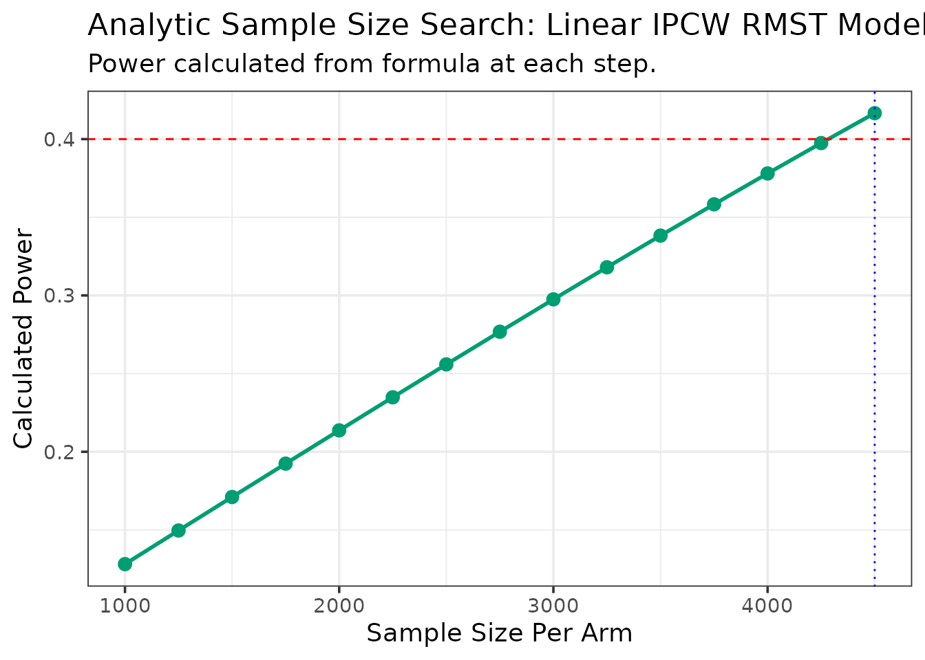
Sample Size Calculation - linear.ss.analytical
We can also use the analytical method to find the required sample size to achieve a target power for a truncation time of one year (365 days).
ss_results_vet <- linear.ss.analytical(
  pilot_data = vet,
  time_var = "time",
  status_var = "status",
  arm_var = "arm",
  target_power = 0.40,
  linear_terms = "karno",
  L = 365,
  n_start = 1000, n_step = 250, max_n_per_arm = 5000
)
--- Estimating parameters from pilot data for analytic search... ---
--- Searching for Sample Size (Method: Analytic) ---
  N = 1000/arm, Calculated Power = 0.128
  N = 1250/arm, Calculated Power = 0.15
  N = 1500/arm, Calculated Power = 0.171
  N = 1750/arm, Calculated Power = 0.192
  N = 2000/arm, Calculated Power = 0.214
  N = 2250/arm, Calculated Power = 0.235
  N = 2500/arm, Calculated Power = 0.256
  N = 2750/arm, Calculated Power = 0.277
  N = 3000/arm, Calculated Power = 0.297
  N = 3250/arm, Calculated Power = 0.318
  N = 3500/arm, Calculated Power = 0.338
  N = 3750/arm, Calculated Power = 0.358
  N = 4000/arm, Calculated Power = 0.378
  N = 4250/arm, Calculated Power = 0.397
  N = 4500/arm, Calculated Power = 0.417

--- Calculation Summary ---


Table: Required Sample Size

| Target_Power| Required_N_per_Arm|
|------------:|------------------:|
| 0.4| 4500|| Statistic | Value | |
|---|---|---|
| factor(arm)1 | Assumed RMST Difference (from pilot) | -3.966558 |
Bootstrap Methods
The .boot suffix in function names indicates a
bootstrap, or simulation-based, approach, which provides a robust,
distribution-free alternative. This method repeatedly resamples from the
pilot data, fits the model on each sample, and calculates power as the
proportion of simulations where the treatment effect is significant.
While computationally intensive, it makes fewer assumptions.
Power and Sample Size Calculation (.boot)
Here is how you would call the bootstrap functions for power for the
linear model. The following examples use the same veteran
dataset, but with a smaller number of simulations for demonstration
purposes. In practice, a larger number of simulations (e.g., 1,000 or
more) is recommended to ensure stable results.
First we calculate the power for a range of sample sizes. The linear.power.boot
function takes the pilot data and returns a data frame with the
estimated power for each sample size.
power_boot_vet <- linear.power.boot(
  pilot_data = vet,
  time_var = "time",
  status_var = "status",
  arm_var = "arm",
  linear_terms = "karno",
  sample_sizes = c(150, 200, 250),
  L = 365,
  n_sim = 200
)
--- Calculating Power (Method: Linear RMST with IPCW) ---
Simulating for n = 150 per arm...
Simulating for n = 200 per arm...
Simulating for n = 250 per arm...

--- Simulation Summary ---


Table: Estimated Treatment Effect (RMST Difference)

|Statistic            |      Value|
|:--------------------|----------:|
|Mean RMST Difference |  -4.087540|
|Mean Standard Error  |   9.161558|
|95% CI Lower         | -24.764020|
|95% CI Upper         |  16.588940|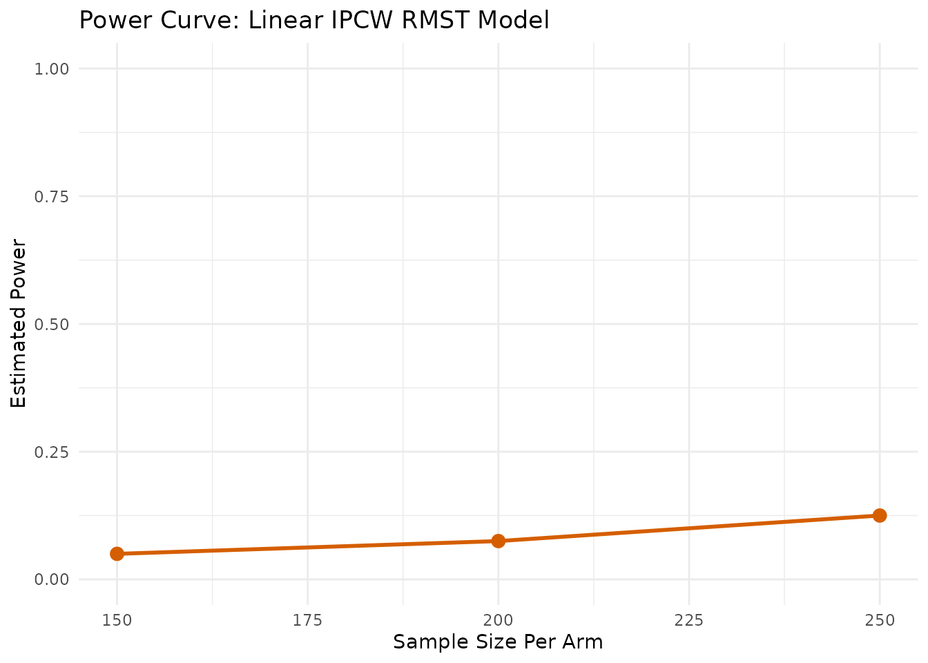
Here is how you would call the bootstrap function for sample size
calculation. We will use the function linear.ss.boot
to find the sample size needed to achieve a target power of 0.5,
truncating at 180 days (6 months).
ss_boot_vet <- linear.ss.boot(
  pilot_data = vet,
  time_var = "time",
  status_var = "status",
  arm_var = "arm",
  target_power = 0.5,
  linear_terms = "karno",
  L = 180,
  n_sim = 500,
  patience = 5
)
--- Searching for Sample Size (Method: Linear RMST with IPCW) ---

--- Searching for N for 50% Power ---
  N = 50/arm, Calculated Power = 0.164
  N = 75/arm, Calculated Power = 0.308
  N = 100/arm, Calculated Power = 0.316
  N = 125/arm, Calculated Power = 0.412
  N = 150/arm, Calculated Power = 0.442
  N = 175/arm, Calculated Power = 0.51

--- Simulation Summary ---


Table: Estimated Treatment Effect (RMST Difference)

|Statistic            |       Value|
|:--------------------|-----------:|
|Mean RMST Difference | -12.0138975|
|Mean Standard Error  |   5.8496564|
|95% CI Lower         | -23.4941297|
|95% CI Upper         |  -0.5336652|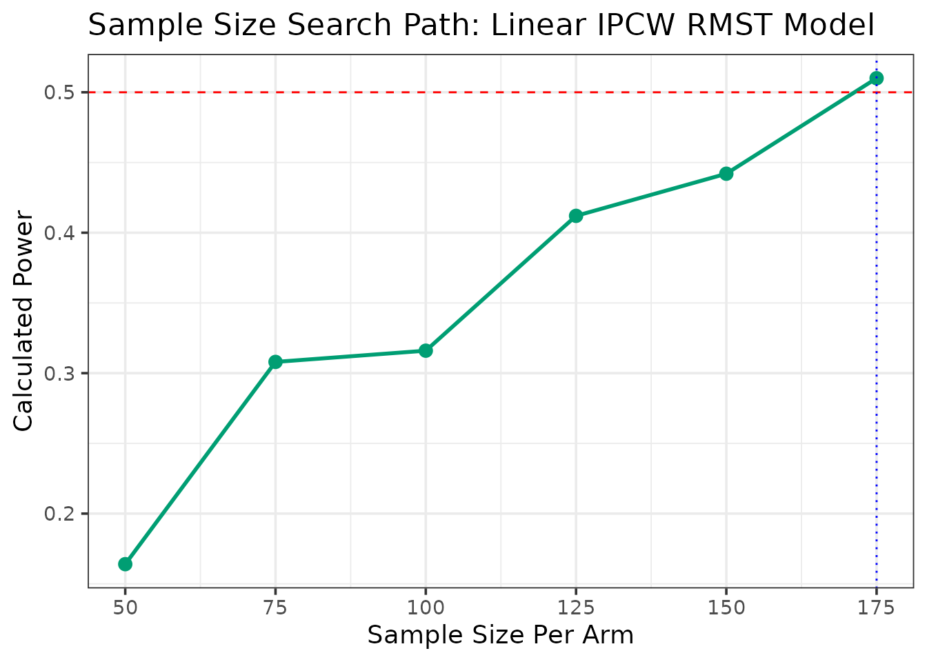
Additive Stratified Models
In multi-center clinical trials, it is often necessary to stratify the analysis by a categorical variable with many levels, such as the clinical center or a discretized biomarker. Estimating a separate parameter for each stratum can be inefficient, particularly when the number of strata is large. The additive stratified model elegantly handles this situation by conditioning out the stratum-specific effects.
Theory and Model
The semiparametric additive model for RMST, as developed by (Zhang and Schaubel 2024), is defined as: This model assumes that the effect of the covariates (which includes the treatment arm) is additive and constant across all strata . Crucially, it allows each stratum to have its own unique baseline RMST, denoted by .
The estimation of the common treatment effect, , is achieved efficiently through a stratum-centering approach applied to IPCW-weighted data. This method avoids the direct estimation of the numerous parameters, making it computationally efficient even with a large number of strata.
Analytical Methods
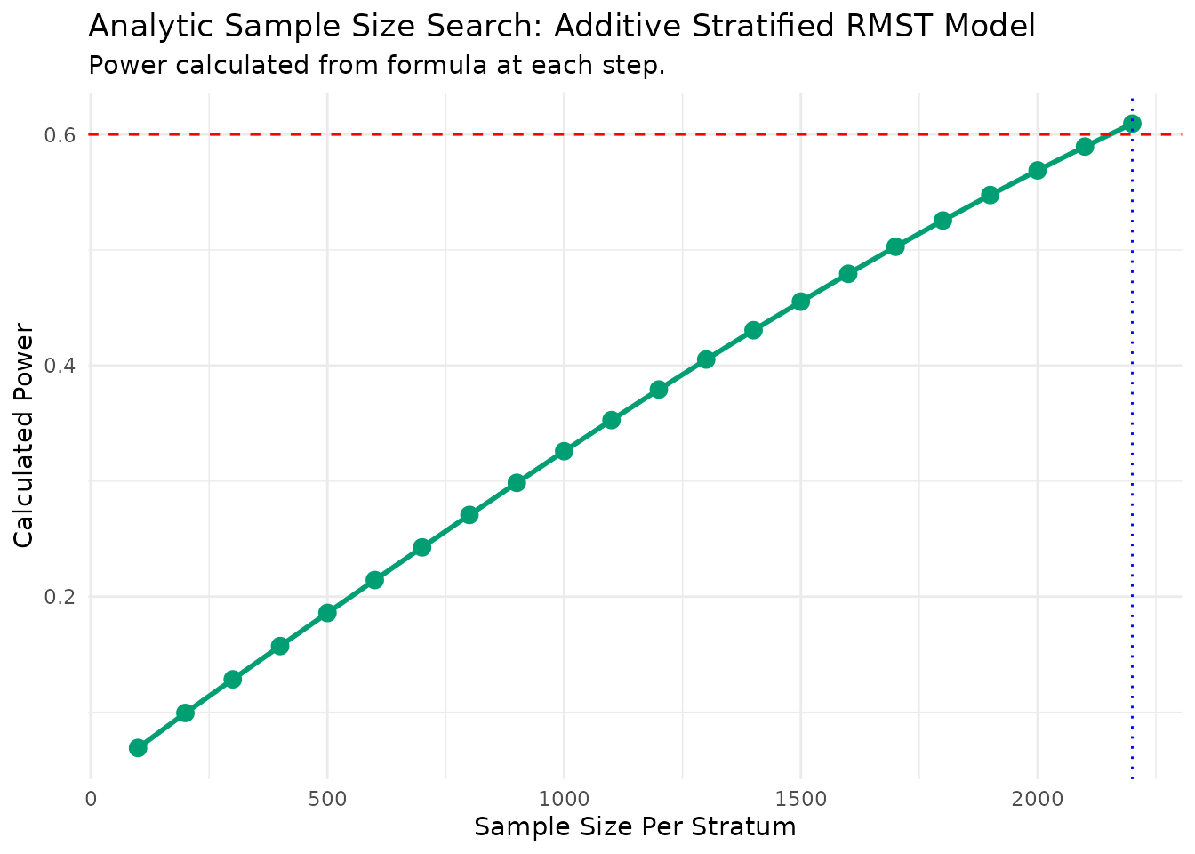
Sample Size Calculation - additive.ss.analytical
Scenario: We use the colon dataset to
design a trial stratified by the extent of local disease
(extent), a factor with 4 levels. We want to find the
sample size per stratum to achieve 80% power. Lets inspect the prepared
colon dataset.
   time status      rx extent arm strata
1  1521      1 Lev+5FU      3   1      3
3  3087      0 Lev+5FU      3   1      3
5   963      1     Obs      2   0      2
7   293      1 Lev+5FU      3   1      3
9   659      1     Obs      3   0      3
11 1767      1 Lev+5FU      3   1      3
Now, we run the sample size search for 80% power, truncating at 5 years (1825 days).
ss_results_colon <- additive.ss.analytical(
  pilot_data = colon_death,
  time_var = "time", status_var = "status", arm_var = "arm", strata_var = "strata",
  target_power = 0.60,
  L = 1825,
  n_start = 100, n_step = 100, max_n_per_arm = 10000
)
--- Estimating parameters from pilot data for analytic search... ---
--- Searching for Sample Size (Method: Additive Analytic) ---
  N = 100/stratum, Calculated Power = 0.069
  N = 200/stratum, Calculated Power = 0.099
  N = 300/stratum, Calculated Power = 0.128
  N = 400/stratum, Calculated Power = 0.157
  N = 500/stratum, Calculated Power = 0.186
  N = 600/stratum, Calculated Power = 0.214
  N = 700/stratum, Calculated Power = 0.243
  N = 800/stratum, Calculated Power = 0.271
  N = 900/stratum, Calculated Power = 0.299
  N = 1000/stratum, Calculated Power = 0.326
  N = 1100/stratum, Calculated Power = 0.353
  N = 1200/stratum, Calculated Power = 0.379
  N = 1300/stratum, Calculated Power = 0.405
  N = 1400/stratum, Calculated Power = 0.431
  N = 1500/stratum, Calculated Power = 0.455
  N = 1600/stratum, Calculated Power = 0.479
  N = 1700/stratum, Calculated Power = 0.503
  N = 1800/stratum, Calculated Power = 0.526
  N = 1900/stratum, Calculated Power = 0.548
  N = 2000/stratum, Calculated Power = 0.569
  N = 2100/stratum, Calculated Power = 0.59
  N = 2200/stratum, Calculated Power = 0.609

--- Calculation Summary ---


Table: Required Sample Size

| Target_Power| Required_N_per_Stratum|
|------------:|----------------------:|
| 0.6| 2200|| Statistic | Value | |
|---|---|---|
| arm | Assumed RMST Difference (from pilot) | -36.77351 |
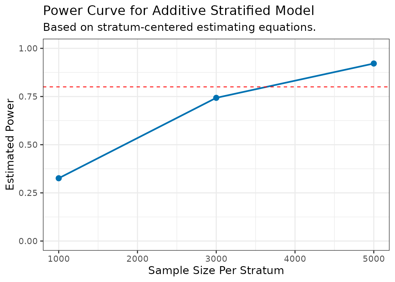
Power Calculation - additive.power.analytical
This function calculates the power for a given set of sample sizes in
a stratified additive model. We will use the colon dataset
again for this example.
power_results_colon <- additive.power.analytical(
  pilot_data = colon_death,
  time_var = "time",
  status_var = "status",
  arm_var = "arm",
  strata_var = "strata",
  sample_sizes = c(1000, 3000, 5000),
  L = 1825 # 5 years
)
--- Estimating parameters from pilot data... ---
--- Estimating additive effect via stratum-centering... ---
--- Calculating asymptotic variance... ---
--- Calculating power for specified sample sizes... ---| N_per_Stratum | Power |
|---|---|
| 1000 | 0.3258947 |
| 3000 | 0.7431725 |
| 5000 | 0.9212546 |
Multiplicative Stratified Models
As an alternative to the additive model, the multiplicative model may be preferred if the treatment is expected to have a relative, or proportional, effect on the RMST—for example, increasing or decreasing survival time by a certain percentage.
Theory and Model
The multiplicative model, based on the work of (Wang et al. 2019), is defined as: In this model, the covariates have a multiplicative effect on the baseline stratum-specific RMST, . This structure is equivalent to a linear model on the log-RMST.
While the formal estimation of
requires a complex iterative solver, this package uses a practical and
computationally efficient approximation. It fits a weighted log-linear
model (lm(log(Y_rmst) ~ ...)) to the data, which provides
robust estimates for the effect size (the log-RMST ratio) and its
variance.
Analytical Methods
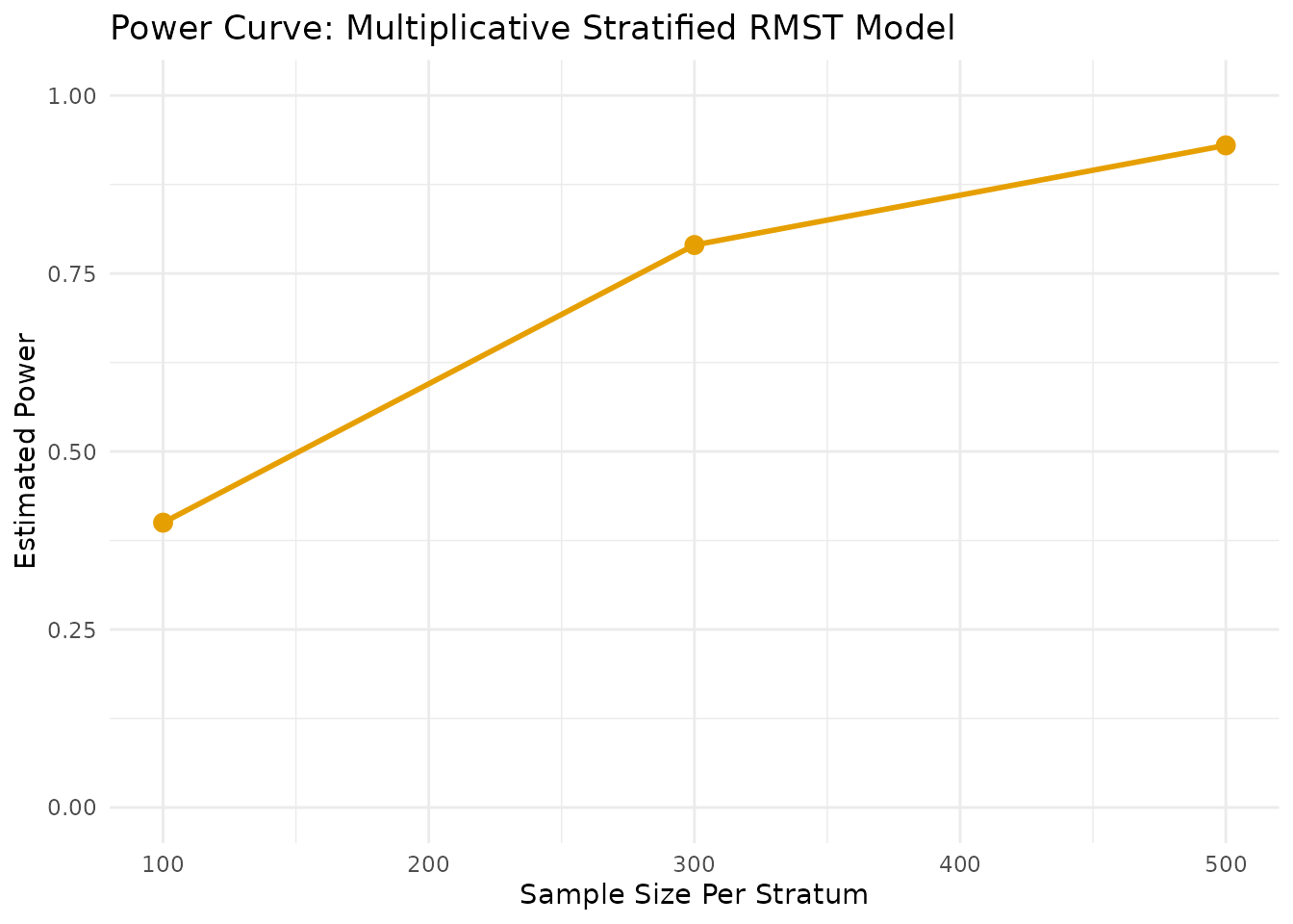
Power Calculation - MS.power.analytical
This function calculates the power for various sample sizes using the analytical method for the multiplicative stratified model.
power_ms_analytical <- MS.power.analytical(
   pilot_data = colon_death,
   time_var = "time", status_var = "status", arm_var = "arm", strata_var = "strata",
   sample_sizes = c(300, 400, 500),
   L = 1825
)
--- Estimating parameters from pilot data (log-linear approximation)... ---
--- Calculating power for specified sample sizes... ---| N_per_Stratum | Power |
|---|---|
| 300 | 0.5061656 |
| 400 | 0.6259153 |
| 500 | 0.7225024 |
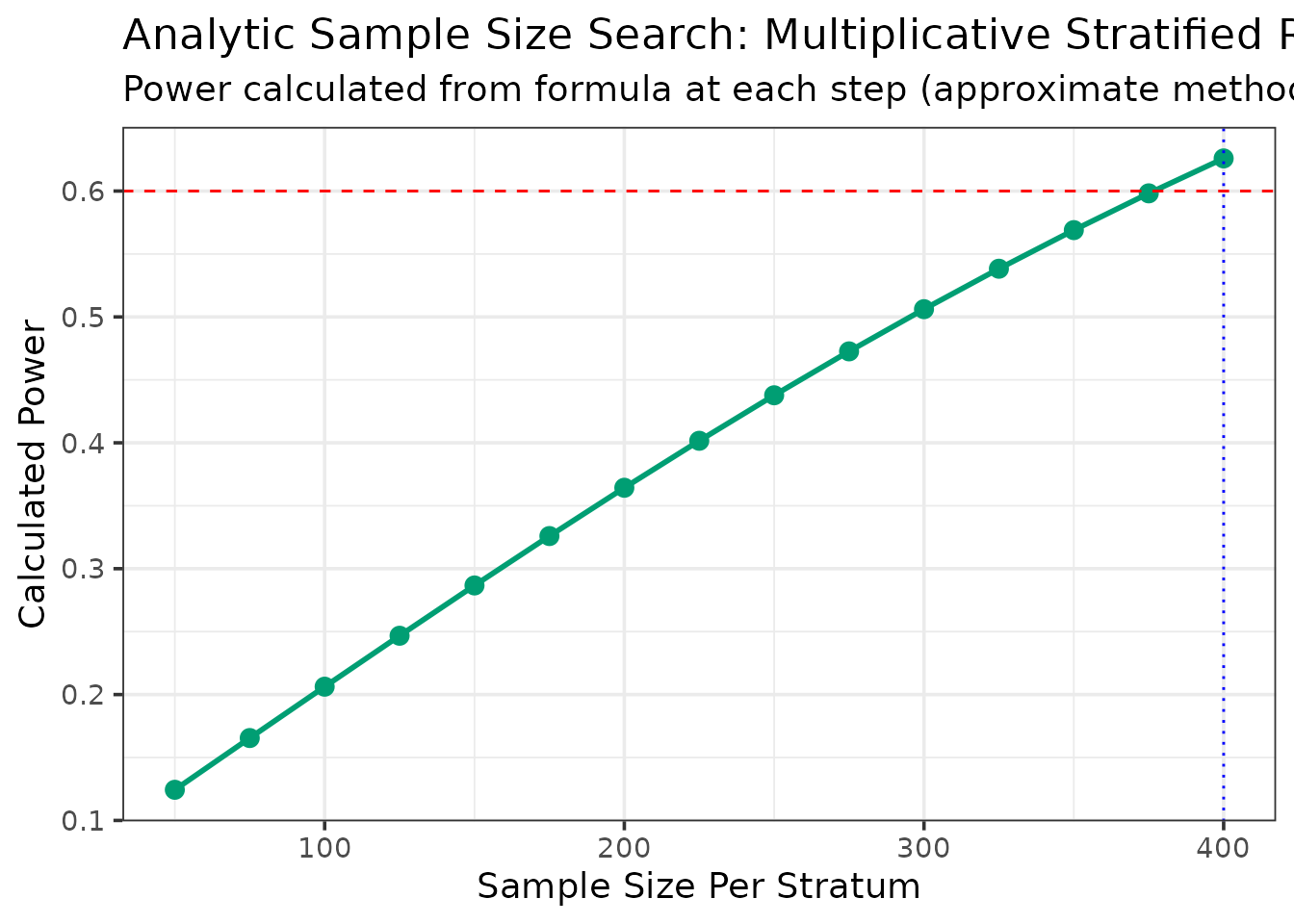
Sample Size Calculation - MS.ss.analytical
The following example demonstrates the sample size calculation using the same model.
ms_ss_results_colon <- MS.ss.analytical(
   pilot_data = colon_death, time_var = "time", status_var = "status", arm_var = "arm", strata_var = "strata",
   target_power = 0.6,L = 1825)
--- Estimating parameters from pilot data (log-linear approximation)... ---
--- Searching for Sample Size (Method: Analytic/Approximation) ---
  N = 50/stratum, Calculated Power = 0.124
  N = 75/stratum, Calculated Power = 0.165
  N = 100/stratum, Calculated Power = 0.206
  N = 125/stratum, Calculated Power = 0.247
  N = 150/stratum, Calculated Power = 0.287
  N = 175/stratum, Calculated Power = 0.326
  N = 200/stratum, Calculated Power = 0.364
  N = 225/stratum, Calculated Power = 0.402
  N = 250/stratum, Calculated Power = 0.438
  N = 275/stratum, Calculated Power = 0.473
  N = 300/stratum, Calculated Power = 0.506
  N = 325/stratum, Calculated Power = 0.538
  N = 350/stratum, Calculated Power = 0.569
  N = 375/stratum, Calculated Power = 0.598
  N = 400/stratum, Calculated Power = 0.626

--- Calculation Summary ---


Table: Required Sample Size

| Target_Power| Required_N_per_Stratum|
|------------:|----------------------:|
| 0.6| 400|| Statistic | Value |
|---|---|
| Assumed log(RMST Ratio) (from pilot) | -0.0898114 |
Bootstrap Methods
The bootstrap approach provides a more robust, simulation-based analysis for the multiplicative model.
Power Calculation - MS.power.boot
The following code demonstrates how to call the
MS.power.boot function.
power_ms_boot <- MS.power.boot(
   pilot_data = colon_death,
   time_var = "time",
   status_var = "status",
   arm_var = "arm",
   strata_var = "strata",
   sample_sizes = c(100, 300, 500),
   L = 1825,
   n_sim = 100,
   parallel.cores = 10
)
--- Calculating Power (Method: Multiplicative Stratified RMST Model) ---
Simulating for n = 100/stratum...
Simulating for n = 300/stratum...
Simulating for n = 500/stratum...

--- Simulation Summary ---


Table: Estimated Treatment Effect (RMST Ratio)

|      |Statistic       |    Value|
|:-----|:---------------|--------:|
|      |Mean RMST Ratio | 1.006522|
|2.5%  |95% CI Lower    | 0.967946|
|97.5% |95% CI Upper | 1.057242|| Statistic | Value | |
|---|---|---|
| Mean RMST Ratio | 1.006522 | |
| 2.5% | 95% CI Lower | 0.967946 |
| 97.5% | 95% CI Upper | 1.057242 |
Sample Size Calculation - MS.ss.boot
Similarly, the sample size can be calculated using bootstrap simulation.
ss_ms_boot <- MS.ss.boot(
   pilot_data = colon_death,
   time_var = "time",
   status_var = "status",
   arm_var = "arm",
   strata_var = "strata",
   target_power = 0.5,
   L = 1825,
   n_sim = 100,
   n_start = 100,
   n_step = 50,
   patience = 4,
   parallel.cores = 10
)
--- Searching for Sample Size (Method: Multiplicative Stratified RMST Model) ---
  N = 100/stratum, Calculating Power...
 Power = 0.35
  N = 150/stratum, Calculating Power...
 Power = 0.5

--- Simulation Summary ---


Table: Estimated Treatment Effect (RMST Ratio)

|      |Statistic       |     Value|
|:-----|:---------------|---------:|
|      |Mean RMST Ratio | 1.0056170|
|2.5%  |95% CI Lower    | 0.9233431|
|97.5% |95% CI Upper | 1.1281975|| Statistic | Value | |
|---|---|---|
| Mean RMST Ratio | 1.0056170 | |
| 2.5% | 95% CI Lower | 0.9233431 |
| 97.5% | 95% CI Upper | 1.1281975 |
Semiparametric GAM Models
When a covariate is expected to have a non-linear effect on the outcome (for example, the effect of age or a biomarker), standard linear models may be misspecified. Generalized Additive Models (GAMs) provide a flexible solution by modeling such relationships with smooth functions.
Theory and Model
These functions use a bootstrap simulation approach combined with a GAM. The method involves two main steps:
Jackknife Pseudo-Observations: The time-to-event outcome is first converted into jackknife pseudo-observations for the RMST. This technique, explored in recent statistical literature for RMST estimation (perdry2024?), creates a continuous, uncensored variable that represents each subject’s contribution to the RMST. This makes the outcome suitable for use in a standard regression framework.
GAM Fitting: A GAM is then fitted to these pseudo-observations. The model has the form: Here, are the non-linear smooth functions (splines) that the GAM estimates from the data.
Power Calculation Formula (GAM.power.boot)
Because this is a bootstrap method, power is not calculated from a direct formula but is instead estimated empirically from the simulations: Where:
is the total number of bootstrap simulations (
n_sim).is the p-value for the treatment effect in the -th simulation.
is the indicator function, which is 1 if the condition is true and 0 otherwise.
Bootstrap Methods
Power Calculation - GAM.power.boot
Scenario: We use the gbsg (German
Breast Cancer Study Group) dataset, suspecting that the progesterone
receptor count (pgr) has a non-linear effect on
recurrence-free survival. Here is a look at the prepared
gbsg data.
   pid age meno size grade nodes pgr er hormon rfstime status arm
1  132  49    0   18     2     2   0  0      0    1838      0   1
2 1575  55    1   20     3    16   0  0      0     403      1   1
3 1140  56    1   40     3     3   0  0      0    1603      0   1
4  769  45    0   25     3     1   0  4      0     177      0   1
5  130  65    1   30     2     5   0 36      1    1855      0   1
6 1642  48    0   52     2    11   0  0      0     842      1   1
The following code shows how to calculate power.
power_gam <- GAM.power.boot(
   pilot_data = gbsg_prepared,
   time_var = "rfstime",
   status_var = "status",
   arm_var = "arm",
   smooth_terms = "pgr", # Model pgr with a smooth term
   sample_sizes = c(50, 200, 400),
   L = 2825, # 5 years
   n_sim = 500,
   parallel.cores = 10
)
--- Calculating Power (Method: Additive GAM for RMST) ---
Simulating for n = 50 /arm ...
Simulating for n = 200 /arm ...
Simulating for n = 400 /arm ...

--- Simulation Summary ---


Table: Estimated Treatment Effect (RMST Difference)

|Statistic            |     Value|
|:--------------------|---------:|
|Mean RMST Difference | 859.57386|
|Mean Standard Error  |  30.44227|
|95% CI Lower         | 796.74021|
|95% CI Upper         | 922.40752|

print(power_gam$results_plot)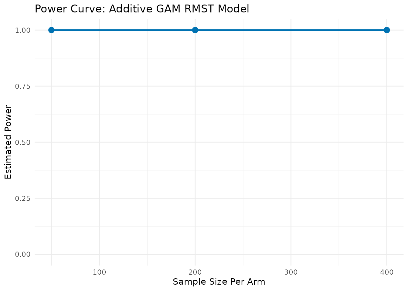
Sample Size Calculation - GAM.ss.boot
Scenario: We want to find the sample size needed to
achieve 80% power for detecting an effect of pgr on
recurrence-free survival.
ss_gam <- GAM.ss.boot(
   pilot_data = gbsg_prepared,
   time_var = "rfstime",
   status_var = "status",
   arm_var = "arm",
   target_power = 0.95,
   L = 182,
   n_sim = 500,
   patience = 5,
   parallel.cores = 10
)
--- Searching for Sample Size (Method: Additive GAM for RMST) ---
  N = 50/arm, Calculating Power... Power = 1

--- Simulation Summary ---


Table: Estimated Treatment Effect (RMST Difference)

|Statistic            |      Value|
|:--------------------|----------:|
|Mean RMST Difference | 90.7118904|
|Mean Standard Error  |  0.2535895|
|95% CI Lower         | 89.7766250|
|95% CI Upper         | 91.6471557|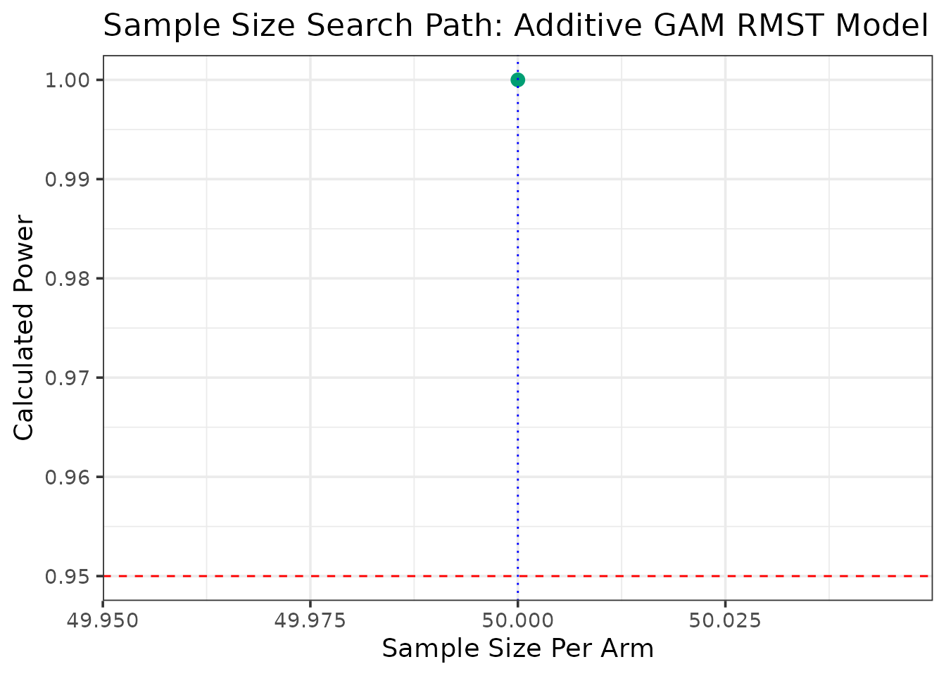
Dependent Censoring Models
In some studies, particularly observational or registry studies, censoring may not be independent of the event of interest. A classic example is in transplant medicine, where receiving an organ transplant removes a patient from being at risk of pre-transplant death. This is a form of competing risk, which can also be viewed as dependent censoring.
Theory and Model
The methods from (Wang and Schaubel 2018) address this by extending the IPCW framework. Instead of a single model for the overall censoring distribution, cause-specific Cox models are fitted for each of the sources of censoring (e.g., one model for administrative censoring, another for the competing event).
The final weight for a subject is then a product of the weights
derived from all censoring causes, calculated as:
where
is the estimated cumulative hazard for censoring cause k,
and
is the truncated event time. The final analysis is a weighted linear
regression on the RMST.
Power Calculation Formula (DC.power.analytical)
Power is calculated analytically using the standard formula: The key difference in this model is that the variance, , is derived from a robust sandwich estimator that properly accounts for the multiple weighting components from the different cause-specific hazard models.
Analytical Methods
We will use the mgus2 dataset for this scenario.
  id age sex dxyr  hgb creat mspike ptime pstat time death event_primary
1  1  88   F 1981 13.1   1.3    0.5    30     0   30     1             0
2  2  78   F 1968 11.5   1.2    2.0    25     0   25     1             0
3  3  94   M 1980 10.5   1.5    2.6    46     0   46     1             0
4  4  68   M 1977 15.2   1.2    1.2    92     0   92     1             0
5  5  90   F 1973 10.7   0.8    1.0     8     0    8     1             0
6  6  90   M 1990 12.9   1.0    0.5     4     0    4     1             0
  event_dependent arm
1               1   0
2               1   0
3               1   1
4               1   1
5               1   0
6               1   1
Power Calculation - DC.power.analytical
This function calculates power for a study with dependent censoring (competing risks) for a given set of sample sizes.
dc_power_results <- DC.power.analytical(
   pilot_data = mgus_prepared,
   time_var = "time",
   status_var = "event_primary",
   arm_var = "arm",
   dep_cens_status_var = "event_dependent",
   sample_sizes = c(100, 250, 500),
   linear_terms = "age",
   L = 120 # 10 years
)
--- Estimating parameters from pilot data... ---
--- Calculating asymptotic variance... ---
--- Calculating power for specified sample sizes... ---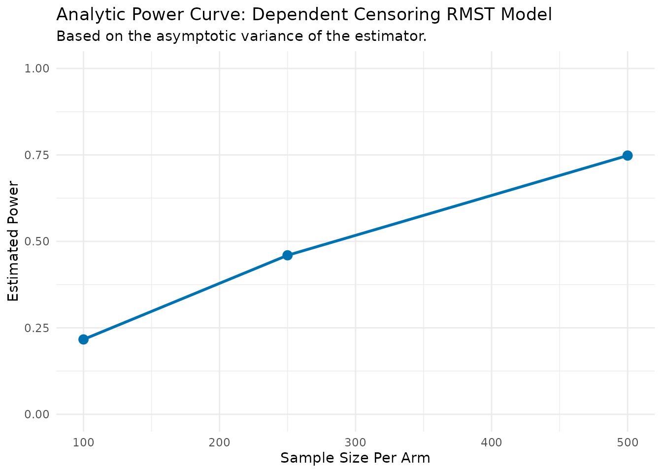
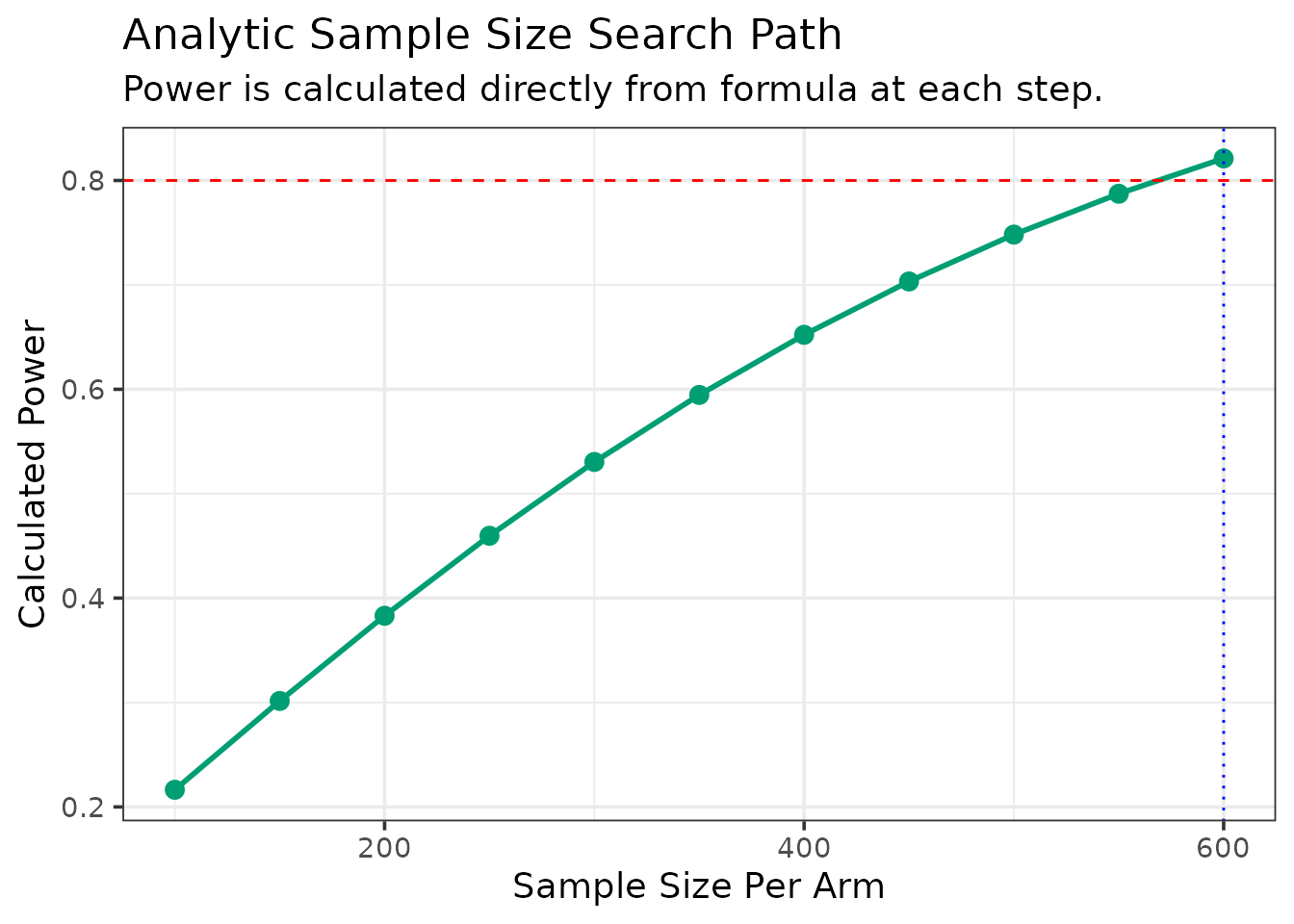
Sample Size Calculation - DC.ss.analytical
Now, find the sample size needed for 80% power, truncating at 10 years (120 months).
ss_dc_mgus <- DC.ss.analytical(
   pilot_data = mgus_prepared,
   time_var = "time",
   status_var = "event_primary",
   arm_var = "arm",
   dep_cens_status_var = "event_dependent",
   target_power = 0.80,
   linear_terms = "age",
   L = 120, # 10 years
   n_start = 100, n_step = 50, max_n_per_arm = 5000
)
--- Estimating parameters from pilot data for analytic calculation... ---
--- Searching for Sample Size (Method: Analytic) ---
  N = 100/arm, Calculated Power = 0.216
  N = 150/arm, Calculated Power = 0.301
  N = 200/arm, Calculated Power = 0.383
  N = 250/arm, Calculated Power = 0.46
  N = 300/arm, Calculated Power = 0.53
  N = 350/arm, Calculated Power = 0.595
  N = 400/arm, Calculated Power = 0.652
  N = 450/arm, Calculated Power = 0.703
  N = 500/arm, Calculated Power = 0.748
  N = 550/arm, Calculated Power = 0.787
  N = 600/arm, Calculated Power = 0.821

--- Calculation Summary ---


Table: Required Sample Size

| Target_Power| Required_N_per_Arm|
|------------:|------------------:|
| 0.8| 600|| Statistic | Value | |
|---|---|---|
| arm | Assumed RMST Difference (from pilot) | 1.556343 |
Interactive Shiny Application
For users who prefer a graphical interface, RMSTSS
provides an interactive Shiny web application that offers a
point-and-click interface to all the models and methods described in
this vignette.
Accessing the Application
There are two ways to access the application:
-
Live Web Version (Recommended): Access the application directly in your browser without any installation.
Run Locally from the R Package: If you have installed the
RMSTSS-Package, you can run the application on your own machine with the following command:
RMSTSS::run_app()App Features
-
Interactive Data Upload: Upload your pilot dataset
in
.csvformat. - Visual Column Mapping: Visually map the columns in your data to the required variables for the analysis (e.g., time, status, treatment arm).
- Full Model Selection: Choose the desired RMST model, calculation method (analytical or bootstrap), and set all relevant parameters through user-friendly controls.
- Rich Visualization: Execute the analysis and view the results, including survival plots, power curves, and summary tables, all within the application.
- Downloadable Reports: Generate and download a complete, publication-ready analysis report in PDF format.
Conclusion
The RMSTSS package provides a powerful and flexible
suite of tools for designing and analyzing clinical trials using the
Restricted Mean Survival Time.
Advantages and Disadvantages
- Advantages: The package implements a wide range of modern statistical methods, allowing users to handle complex scenarios like stratification, non-linear effects, and competing risks. The provision of both fast analytical methods and robust bootstrap methods gives users a choice between speed and distributional flexibility.
- Disadvantages: The primary limitation is the reliance on representative pilot data. The accuracy of any power or sample size calculation is contingent on the effect sizes and variance structures estimated from the pilot dataset. Furthermore, the bootstrap-based methods can be computationally intensive and may require access to parallel computing resources for timely results.