Analyze Power for a Stratified Additive RMST Model (Analytic)

Performs power analysis for a stratified, additive RMST model using the analytic variance estimator based on the method of Zhang & Schaubel (2024).

Usage

additive.power.analytical(
  pilot_data,
  time_var,
  status_var,
  arm_var,
  strata_var,
  sample_sizes,
  linear_terms = NULL,
  L,
  alpha = 0.05
)

Arguments

pilot_data: A data.frame containing pilot study data.
time_var: A character string for the time-to-event variable.
status_var: A character string for the event status variable (1=event, 0=censored).
arm_var: A character string for the treatment arm variable (1=treatment, 0=control).
strata_var: A character string for the stratification variable.
sample_sizes: A numeric vector of sample sizes per stratum to calculate power for.
linear_terms: An optional character vector of other covariate names.
L: The numeric value for the RMST truncation time.
alpha: The significance level (Type I error rate).

Value

A list containing:

results_data: A data.frame with specified sample sizes and corresponding powers.
results_plot: A ggplot object visualizing the power curve.

Details

This function implements the power calculation for the semiparametric additive model for RMST, given by \(\mu_{ij} = \mu_{0j} + \beta'Z_i\), where i is the subject and j is the stratum.

The method uses Inverse Probability of Censoring Weighting (IPCW), where weights are derived from a stratified Cox model on the censoring times. The regression coefficient \(\hat{\beta}\) is estimated using a closed-form solution that involves centering the covariates and RMST values within each stratum.

Power is determined analytically from the asymptotic sandwich variance of \(\hat{\beta}\). This implementation uses a robust variance estimator of the form \(A_n^{-1} B_n (A_n^{-1})'\), where \(A_n\) and \(B_n\) are empirical estimates of the variance components.

Examples

set.seed(123)
pilot_df_strat <- data.frame(
 time = rexp(150, 0.1),
 status = rbinom(150, 1, 0.8),
 arm = rep(0:1, each = 75),
 region = factor(rep(c("A", "B", "C"), each = 50)),
 age = rnorm(150, 60, 10)
)
# Introduce an additive treatment effect
pilot_df_strat$time[pilot_df_strat$arm == 1] <-
  pilot_df_strat$time[pilot_df_strat$arm == 1] + 1.5

power_results <- additive.power.analytical(
  pilot_data = pilot_df_strat,
  time_var = "time", status_var = "status", arm_var = "arm", strata_var = "region",
  sample_sizes = c(100, 150, 200),
  linear_terms = "age",
  L = 12
)
#> --- Estimating parameters from pilot data... ---
#> --- Estimating additive effect via stratum-centering... ---
#> --- Calculating asymptotic variance... ---
#> --- Calculating power for specified sample sizes... ---
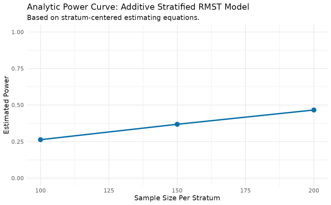
print(power_results$results_data)
#>   N_per_Stratum     Power
#> 1           100 0.2629389
#> 2           150 0.3682932
#> 3           200 0.4660482
print(power_results$results_plot)