RMSTpowerBoost: Sample Size and Power Calculations for RMST-based Clinical Trials

Introduction

Clinical trials with time-to-event endpoints often rely on hazard-based methods such as the proportional hazards (PH) model and the hazard ratio (HR). The HR can be hard to interpret when treatment effects vary over time, and the proportional hazards assumption is frequently violated in practice.

The Restricted Mean Survival Time (RMST) is the expected event-free time up to a pre-specified follow-up point, $L$(Royston and Parmar 2013; Uno et al. 2014). It yields a treatment contrast on the time scale, such as an average gain of several months over a clinically relevant horizon.

Recent work models RMST directly as a function of baseline covariates instead of estimating it only from a survival curve or hazard model. Methods based on Inverse Probability of Censoring Weighting (IPCW) (Tian et al. 2014) now cover stratified studies (Wang et al. 2019; Zhang and Schaubel 2024) and covariate-dependent censoring (Wang and Schaubel 2018).

Most available software emphasizes estimation from existing data rather than study design. As a result, trial statisticians often need custom code for sample size and power calculations.

RMSTpowerBoost implements direct RMST methods for power and sample size calculations:

• Linear IPCW Models: A direct regression model for RMST with IPCW-based estimation (Tian et al. 2014).
• Stratified Models: Efficient methods for studies with a large number of strata (e.g., clinical centers), including both additive (Zhang and Schaubel 2024) and multiplicative (Wang et al. 2019) models.
• Dependent Censoring Models: Methods for handling covariate-dependent censoring (Wang and Schaubel 2018).
• Flexible Non-Linear Models: Bootstrap-based functions using Generalized Additive Models (GAMs) to capture non-linear covariate effects.
• Analytic vs. Bootstrap Methods: For most models, the package offers a choice between a fast analytical calculation and a simulation-based boot method.

This vignette outlines the main model families and shows how to use them.

---

Core Concepts of RMSTpowerBoost Package

The functions in this package are grounded in a regression-based formulation of the restricted mean survival time (RMST). For a given subject $i$ with event time $T_i$, covariate vector $Z_i$ and treatment indicator $\mathrm{Trt}_i$, the conditional RMST is modeled as

$$\mathbb{E}[\min(T_i, L)\mid Z_i] \;=\; \beta_0 + \beta_{\text{effect}}\,\mathrm{Trt}_i + \beta_2^{\top} Z_i,$$

where $L$ is the restriction time, and $\beta_{\text{effect}}$ represents the modeled treatment contrast on the RMST scale, that is, the expected difference in event-free time between treatment arms after adjustment for the included covariates. The quantity $\beta_{\text{effect}}$ therefore defines the effect size used throughout the analytical power and sample size functions in RMSTpowerBoost.

The Analytic Method

The analytical functions estimate power from a closed-form expression, so they are useful for rapid scenario exploration. The process is:

1. One-Time Estimation: The function first analyzes the provided reference data to estimate two key parameters:
   • The treatment effect size (e.g., the difference in RMST or the log-RMST ratio).
   • The asymptotic variance of that effect estimator, which measures its uncertainty.
2. Power Formula: It then plugs these fixed estimates into a standard power formula. For a given total sample size N, the power is calculated as: $$\text{Power} = \Phi\left( \frac{|\beta_{\text{effect}}|}{\sigma_N} - z_{1-\alpha/2} \right)$$ where:
   • $\Phi$ is the cumulative distribution function (CDF) of the standard normal distribution.
   • $\beta_{\text{effect}}$ is the treatment effect.
   • $\sigma_N = \frac{\sigma_1}{\sqrt{N}}$ is the standard error of the effect for the target sample size N, which is scaled from the reference data’s variance.
   • $z_{1-\alpha/2}$ is the critical value from the standard normal distribution (e.g., 1.96 for an alpha of 0.05).

The Bootstrap Method

The bootstrap functions estimate power empirically and therefore require more computation. The process is:

1. Resample: The function simulates a “future trial” of a given sample_size by resampling with replacement from the reference data.
2. Fit Model: On this new bootstrap sample, it performs the full analysis (e.g., calculating weights or pseudo-observations and fitting the specified model).
3. Get P-Value: It extracts the p-value for the treatment effect from the fitted model.
4. Repeat: This process is repeated thousands of times (n_sim).
5. Calculate Power: The final estimated power is the proportion of simulations where the p-value was less than the significance level alpha. $$\text{Power} = \frac{\text{Number of simulations with } p < \alpha}{n_{\text{sim}}}$$

The Sample Size Search Algorithm

rmst.ss() uses an iterative search algorithm to find the N required to achieve a target_power:

1. Start: The search begins with a sample size of n_start.
2. Calculate Power: It calculates the power for the current_n using either the analytic formula or a full bootstrap simulation.
3. Check Condition:
   • If calculated_power >= target_power, the search succeeds and returns current_n.
   • If not, it increments the sample size (current_n = current_n + n_step) and repeats the process.
4. Stopping Rules: The search terminates if the sample size exceeds max_n or, for bootstrap methods, if the power fails to improve for a set number of patience steps.

The Unified Interface

RMSTpowerBoost exposes all models through two top-level functions that use a familiar Surv()-based formula interface:

Function	Purpose
rmst.power(Surv(time, status) ~ covariates, data, arm, sample_sizes, L, ...)	Power curve over a vector of sample sizes
rmst.ss(Surv(time, status) ~ covariates, data, arm, target_power, L, ...)	Minimum sample size to reach a power target

Key arguments that control model selection:

Argument	Values	Effect
type	"analytical" (default) / "boot"	Analytic vs. bootstrap method
strata	column name / ~col / NULL	Activates stratified model
strata_type	"additive" / "multiplicative"	Stratified model type
dep_cens	TRUE / FALSE	Dependent-censoring model
Smooth terms	s(var) in formula	Activates GAM (forces type = "boot")

The underlying model-specific functions remain exported for direct use when needed.

Selecting an Appropriate Model

Model choice depends on the study design and the assumptions you are willing to make. The table below summarizes typical settings for each approach:

Model	Key Assumption / Scenario	Use when
Linear IPCW	Assumes a linear relationship between covariates and RMST.	there is no strong evidence of non-linear effects or complex stratification.
Additive Stratified	Assumes the treatment adds a constant amount of survival time across strata.	treatment effects are expected to be comparable across centers or other strata.
Multiplicative Stratified	Assumes the treatment multiplies survival time proportionally across strata.	treatment effects are better expressed as relative changes in RMST across strata.
Semiparametric GAM	Allows for non-linear covariate effects on RMST.	covariates such as age or biomarkers are likely to have non-linear associations with the outcome.
Dependent Censoring	Accounts for covariate-dependent censoring under a single censoring mechanism.	censoring depends on measured covariates and competing risks are not being modeled explicitly.

Linear IPCW Models

These functions implement the foundational direct linear regression model for the RMST. This model is appropriate when a linear relationship between covariates and the RMST is assumed, and when censoring is independent of the event of interest.

Theory and Model

Based on the methods of (Tian et al. 2014), these functions model the conditional RMST as a linear function of covariates: $$\mathbb{E}[\min(T_i, L) | Z_i] = \beta_0 + \beta_{\text{effect}} \text{Treatment}_i + \beta_2 \text{Covariate}_{i}$$ In this model, the expected RMST up to a pre-specified time L for subject i is modeled as a linear combination of their treatment arm and other variables $Z_i$.

To handle right-censoring, the method uses Inverse Probability of Censoring Weighting (IPCW). This is achieved through the following steps:

1. A survival curve for the censoring distribution is estimated using the Kaplan-Meier method (where “failure” is being censored).
2. For each subject who experienced the primary event, a weight is calculated. This weight is the inverse of the probability of not being censored up to their event time.
3. A standard weighted linear model (lm()) is then fitted using these weights. The model only includes subjects who experienced the event.

Analytical Methods

The analytical functions use a formula based on the asymptotic variance of the regression coefficients to calculate power or sample size, making them fast to evaluate.

Scenario: We use the veteran dataset to estimate power for a trial comparing standard vs. test chemotherapy (trt), adjusting for the Karnofsky performance score (karno).

Power Calculation

First, let’s inspect the prepared veteran dataset.

  trt celltype time status karno diagtime age prior arm
1   1 squamous   72      1    60        7  69     0   0
2   1 squamous  411      1    70        5  64    10   0
3   1 squamous  228      1    60        3  38     0   0
4   1 squamous  126      1    60        9  63    10   0
5   1 squamous  118      1    70       11  65    10   0
6   1 squamous   10      1    20        5  49     0   0

Now, we calculate the power for a range of sample sizes using a truncation time of 9 months (270 days).

power_results_vet <- rmst.power(
  Surv(time, status) ~ karno,
  data         = vet,
  arm          = "arm",
  sample_sizes = c(100, 150, 200, 250),
  L            = 270
)
--- Estimating parameters from pilot data for analytic calculation... ---
--- Calculating asymptotic variance... ---
--- Calculating power for specified sample sizes... ---

The results are returned as a data frame and a ggplot object.

Power Analysis for Veteran Dataset

N_per_Arm	Power
100	0.1265610
150	0.1687428
200	0.2106066
250	0.2520947

Sample Size Calculation

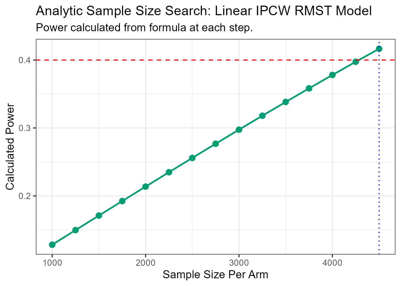
We can also use the analytical method to find the required sample size to achieve a target power for a truncation time of one year (365 days).

ss_results_vet <- rmst.ss(
  Surv(time, status) ~ karno,
  data         = vet,
  arm          = "arm",
  target_power = 0.40,
  L            = 365,
  n_start = 1000, n_step = 250, max_n = 5000
)
--- Estimating parameters from pilot data for analytic search... ---
--- Searching for Sample Size (Method: Analytic) ---
  N = 1000/arm, Calculated Power = 0.128
  N = 1250/arm, Calculated Power = 0.15
  N = 1500/arm, Calculated Power = 0.171
  N = 1750/arm, Calculated Power = 0.192
  N = 2000/arm, Calculated Power = 0.214
  N = 2250/arm, Calculated Power = 0.235
  N = 2500/arm, Calculated Power = 0.256
  N = 2750/arm, Calculated Power = 0.277
  N = 3000/arm, Calculated Power = 0.297
  N = 3250/arm, Calculated Power = 0.318
  N = 3500/arm, Calculated Power = 0.338
  N = 3750/arm, Calculated Power = 0.358
  N = 4000/arm, Calculated Power = 0.378
  N = 4250/arm, Calculated Power = 0.397
  N = 4500/arm, Calculated Power = 0.417

--- Calculation Summary ---


Table: Required Sample Size

| Target_Power| Required_N_per_Arm|
|------------:|------------------:|
|          0.4|               4500|

Estimated Effect from Reference Data

	Statistic	Value
factor(arm)1	Assumed RMST Difference (from pilot)	-3.966558

Bootstrap Methods

Passing type = "boot" to rmst.power() or rmst.ss() switches to a simulation-based approach. This method repeatedly resamples from the reference data, fits the model on each sample, and calculates power as the proportion of simulations where the treatment effect is significant. It relies less on closed-form large-sample approximations at the cost of greater computation time.

Power and Sample Size Calculation (bootstrap)

Here is how you would call the bootstrap method for power for the linear model. The following examples use the same veteran dataset, but with a smaller number of simulations for demonstration purposes. In practice, a larger number of simulations (e.g., 1,000 or more) is recommended to ensure stable results.

First we calculate the power for a range of sample sizes.

power_boot_vet <- rmst.power(
  Surv(time, status) ~ karno,
  data         = vet,
  arm          = "arm",
  sample_sizes = c(150, 200, 250),
  L            = 365,
  type         = "boot",
  n_sim        = 50
)
--- Calculating Power (Method: Linear RMST with IPCW) ---
Simulating for n = 150 per arm...
Simulating for n = 200 per arm...
Simulating for n = 250 per arm...

--- Simulation Summary ---


Table: Estimated Treatment Effect (RMST Difference)

|Statistic            |      Value|
|:--------------------|----------:|
|Mean RMST Difference |  -3.366849|
|Mean Standard Error  |   9.092000|
|95% CI Lower         | -21.050205|
|95% CI Upper         |  14.316506|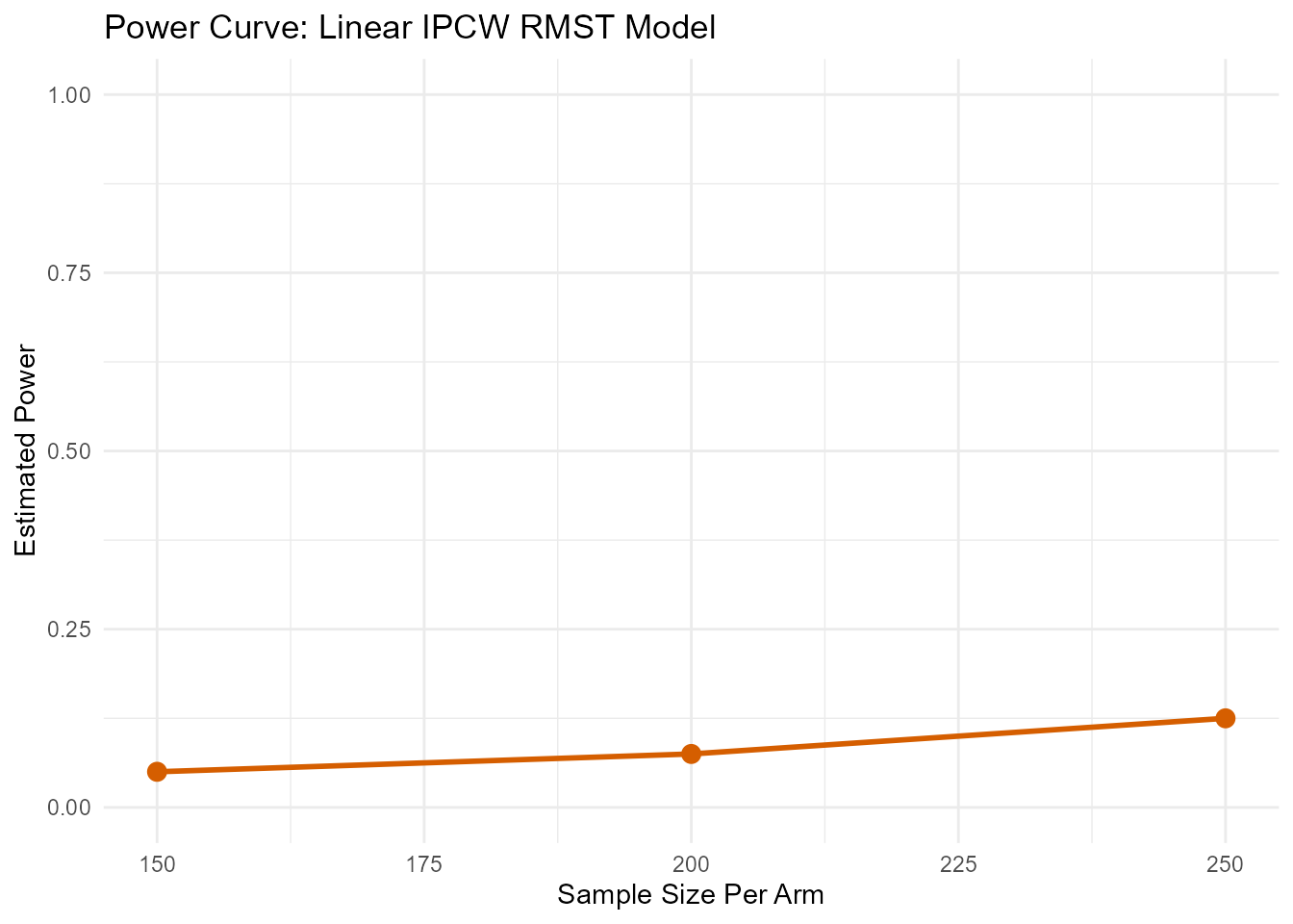

Here is how you would call the bootstrap method for sample size calculation, targeting 50% power and truncating at 180 days (6 months).

ss_boot_vet <- rmst.ss(
  Surv(time, status) ~ karno,
  data         = vet,
  arm          = "arm",
  target_power = 0.5,
  L            = 180,
  type         = "boot",
  n_sim        = 100,
  patience     = 5
)
--- Searching for Sample Size (Method: Linear RMST with IPCW) ---

--- Searching for N for 50% Power ---
  N = 50/arm, Calculated Power = 0.27
  N = 75/arm, Calculated Power = 0.22
  N = 100/arm, Calculated Power = 0.4
  N = 125/arm, Calculated Power = 0.44
  N = 150/arm, Calculated Power = 0.41
  N = 175/arm, Calculated Power = 0.51

--- Simulation Summary ---


Table: Estimated Treatment Effect (RMST Difference)

|Statistic            |       Value|
|:--------------------|-----------:|
|Mean RMST Difference | -11.3968671|
|Mean Standard Error  |   5.8217038|
|95% CI Lower         | -22.6513793|
|95% CI Upper         |  -0.1423548|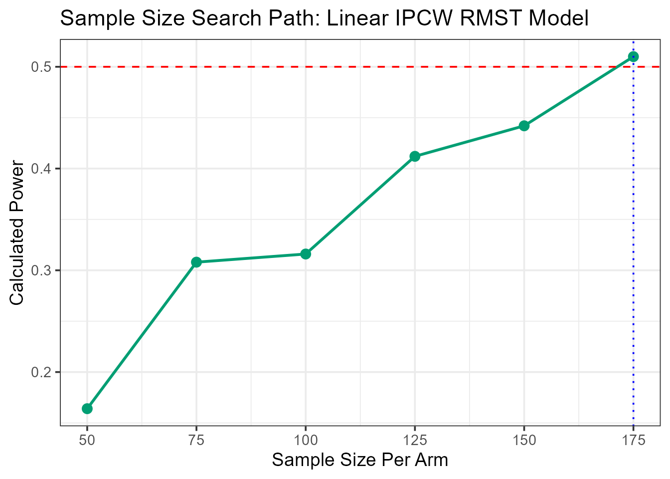

---

Additive Stratified Models

In multi-center clinical trials, the analysis is often stratified by a categorical variable with many levels, such as clinical center or a discretized biomarker. Estimating a separate parameter for each stratum can be inefficient when the number of strata is large. The additive stratified model removes the stratum-specific effects through conditioning.

Theory and Model

The semiparametric additive model for RMST, as developed by (Zhang and Schaubel 2024), is defined as: $$\mu_{ij} = \mu_{0j} + \beta'Z_i$$ This model assumes that the effect of the covariates $Z_i$ (which includes the treatment arm) is additive and constant across all strata $j$. Each stratum has its own baseline RMST, denoted by $\mu_{0j}$.

The common treatment effect, $\beta$, is estimated with a stratum-centering approach applied to IPCW-weighted data. This avoids direct estimation of the many $\mu_{0j}$ parameters.

Analytical Methods

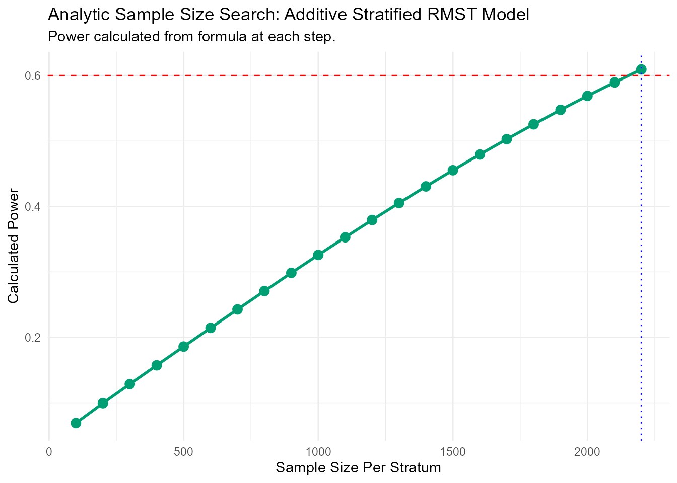
Sample Size Calculation

Scenario: We use the colon dataset to design a trial stratified by the extent of local disease (extent), a factor with 4 levels. We want to find the sample size per stratum to achieve 60% power. Let’s inspect the prepared colon dataset.

   time status      rx extent arm strata
1  1521      1 Lev+5FU      3   1      3
3  3087      0 Lev+5FU      3   1      3
5   963      1     Obs      2   0      2
7   293      1 Lev+5FU      3   1      3
9   659      1     Obs      3   0      3
11 1767      1 Lev+5FU      3   1      3

Now, we run the sample size search for 60% power, truncating at 5 years (1825 days).

ss_results_colon <- rmst.ss(
  Surv(time, status) ~ 1,
  data         = colon_death,
  arm          = "arm",
  strata       = "strata",
  strata_type  = "additive",
  target_power = 0.60,
  L            = 1825,
  n_start = 100, n_step = 100, max_n = 10000
)
--- Estimating parameters from pilot data for analytic search... ---
--- Searching for Sample Size (Method: Additive Analytic) ---
  N = 100/stratum, Calculated Power = 0.069
  N = 200/stratum, Calculated Power = 0.099
  N = 300/stratum, Calculated Power = 0.128
  N = 400/stratum, Calculated Power = 0.157
  N = 500/stratum, Calculated Power = 0.186
  N = 600/stratum, Calculated Power = 0.214
  N = 700/stratum, Calculated Power = 0.243
  N = 800/stratum, Calculated Power = 0.271
  N = 900/stratum, Calculated Power = 0.299
  N = 1000/stratum, Calculated Power = 0.326
  N = 1100/stratum, Calculated Power = 0.353
  N = 1200/stratum, Calculated Power = 0.379
  N = 1300/stratum, Calculated Power = 0.405
  N = 1400/stratum, Calculated Power = 0.431
  N = 1500/stratum, Calculated Power = 0.455
  N = 1600/stratum, Calculated Power = 0.479
  N = 1700/stratum, Calculated Power = 0.503
  N = 1800/stratum, Calculated Power = 0.526
  N = 1900/stratum, Calculated Power = 0.548
  N = 2000/stratum, Calculated Power = 0.569
  N = 2100/stratum, Calculated Power = 0.59
  N = 2200/stratum, Calculated Power = 0.609

--- Calculation Summary ---


Table: Required Sample Size

| Target_Power| Required_N_per_Stratum|
|------------:|----------------------:|
|          0.6|                   2200|

Estimated Effect from Reference Data

	Statistic	Value
arm	Assumed RMST Difference (from pilot)	-36.77351

Power Calculation

This example calculates the power for a given set of sample sizes in a stratified additive model using the same colon dataset.

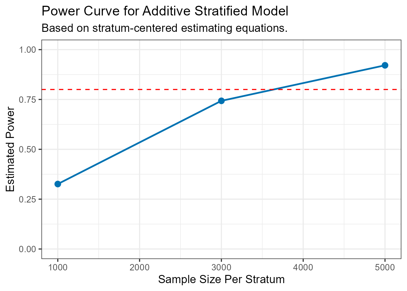
power_results_colon <- rmst.power(
  Surv(time, status) ~ 1,
  data         = colon_death,
  arm          = "arm",
  strata       = "strata",
  strata_type  = "additive",
  sample_sizes = c(1000, 3000, 5000),
  L            = 1825
)
--- Estimating parameters from pilot data... ---
--- Estimating additive effect via stratum-centering... ---
--- Calculating asymptotic variance... ---
--- Calculating power for specified sample sizes... ---

Power for Additive Stratified Colon Trial

N_per_Stratum	Power
1000	0.3258947
3000	0.7431725
5000	0.9212546

---

Multiplicative Stratified Models

Use the multiplicative model when treatment is expected to act on the RMST scale through a relative effect, such as a percentage increase or decrease in survival time.

Theory and Model

The multiplicative model, based on the work of (Wang et al. 2019), is defined as: $$\mu_{ij} = \mu_{0j} \exp(\beta'Z_i)$$ In this model, the covariates $Z_i$ have a multiplicative effect on the baseline stratum-specific RMST, $\mu_{0j}$. This structure is equivalent to a linear model on the log-RMST.

Formal estimation of $\beta$ requires an iterative solver. This package instead fits a weighted log-linear model (lm(log(Y_rmst) ~ ...)) to approximate the log-RMST ratio and its variance.

Analytical Methods

Power Calculation

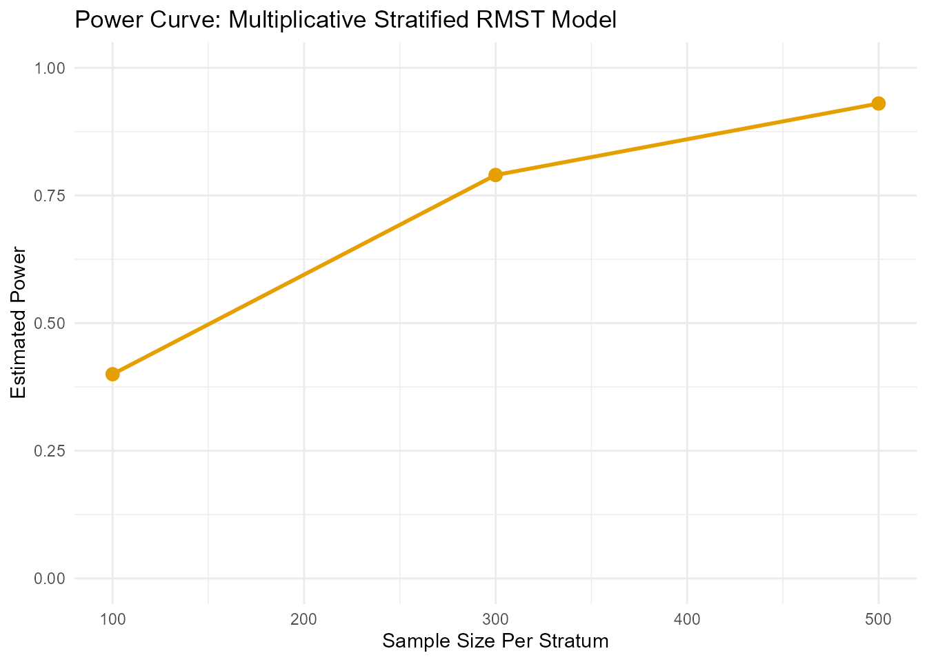
This function calculates the power for various sample sizes using the analytical method for the multiplicative stratified model.

power_ms_analytical <- rmst.power(
  Surv(time, status) ~ 1,
  data         = colon_death,
  arm          = "arm",
  strata       = "strata",
  strata_type  = "multiplicative",
  sample_sizes = c(300, 400, 500),
  L            = 1825
)
--- Estimating parameters from pilot data (log-linear approximation)... ---
--- Calculating power for specified sample sizes... ---

Power for Multiplicative Stratified Model

N_per_Stratum	Power
300	0.5061656
400	0.6259153
500	0.7225024

Sample Size Calculation

The following example demonstrates the sample size calculation for the multiplicative model.

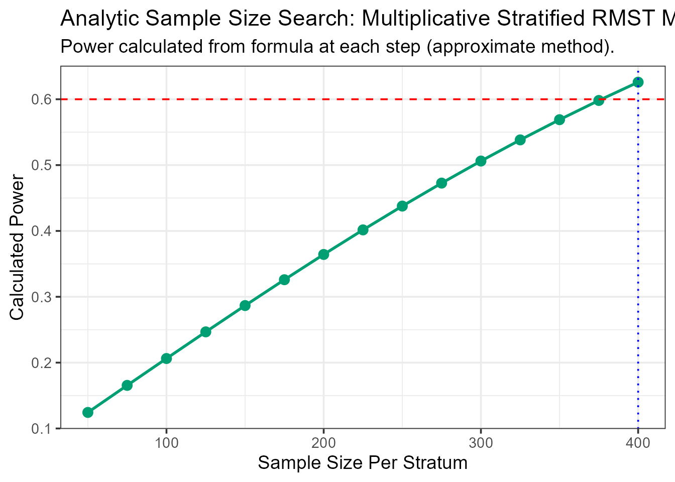
ms_ss_results_colon <- rmst.ss(
  Surv(time, status) ~ 1,
  data         = colon_death,
  arm          = "arm",
  strata       = "strata",
  strata_type  = "multiplicative",
  target_power = 0.6,
  L            = 1825
)
--- Estimating parameters from pilot data (log-linear approximation)... ---
--- Searching for Sample Size (Method: Analytic/Approximation) ---
  N = 50/stratum, Calculated Power = 0.124
  N = 75/stratum, Calculated Power = 0.165
  N = 100/stratum, Calculated Power = 0.206
  N = 125/stratum, Calculated Power = 0.247
  N = 150/stratum, Calculated Power = 0.287
  N = 175/stratum, Calculated Power = 0.326
  N = 200/stratum, Calculated Power = 0.364
  N = 225/stratum, Calculated Power = 0.402
  N = 250/stratum, Calculated Power = 0.438
  N = 275/stratum, Calculated Power = 0.473
  N = 300/stratum, Calculated Power = 0.506
  N = 325/stratum, Calculated Power = 0.538
  N = 350/stratum, Calculated Power = 0.569
  N = 375/stratum, Calculated Power = 0.598
  N = 400/stratum, Calculated Power = 0.626

--- Calculation Summary ---


Table: Required Sample Size

| Target_Power| Required_N_per_Stratum|
|------------:|----------------------:|
|          0.6|                    400|

Sample Size for Multiplicative Stratified Model

Statistic	Value
Assumed log(RMST Ratio) (from pilot)	-0.0898114

Bootstrap Methods

The bootstrap approach provides a simulation-based analysis for the multiplicative model. Pass type = "boot" together with strata_type = "multiplicative".

Power Calculation (bootstrap)

power_ms_boot <- rmst.power(
  Surv(time, status) ~ 1,
  data           = colon_death,
  arm            = "arm",
  strata         = "strata",
  strata_type    = "multiplicative",
  sample_sizes   = c(100, 300, 500),
  L              = 1825,
  type           = "boot",
  n_sim          = 30,
  parallel.cores = 1
)
--- Calculating Power (Method: Multiplicative Stratified RMST Model) ---
Simulating for n = 100/stratum...
Simulating for n = 300/stratum...
Simulating for n = 500/stratum...

--- Simulation Summary ---


Table: Estimated Treatment Effect (RMST Ratio)

|      |Statistic       |     Value|
|:-----|:---------------|---------:|
|      |Mean RMST Ratio | 1.0077347|
|2.5%  |95% CI Lower    | 0.9565007|
|97.5% |95% CI Upper    | 1.0564916|

Power for Multiplicative Stratified Model (Bootstrap)

	Statistic	Value
	Mean RMST Ratio	1.0077347
2.5%	95% CI Lower	0.9565007
97.5%	95% CI Upper	1.0564916

Sample Size Calculation (bootstrap)

ss_ms_boot <- rmst.ss(
  Surv(time, status) ~ 1,
  data           = colon_death,
  arm            = "arm",
  strata         = "strata",
  strata_type    = "multiplicative",
  target_power   = 0.75,
  L              = 1825,
  type           = "boot",
  n_sim          = 30,
  n_start        = 100,
  n_step         = 50,
  patience       = 4,
  parallel.cores = 1
)
--- Searching for Sample Size (Method: Multiplicative Stratified RMST Model) ---
  N = 100/stratum, Calculating Power... Power = 0.433
  N = 150/stratum, Calculating Power... Power = 0.733
  N = 200/stratum, Calculating Power... Power = 0.6
  N = 250/stratum, Calculating Power... Power = 0.6
  N = 300/stratum, Calculating Power... Power = 0.733
  N = 350/stratum, Calculating Power... Power = 0.8

--- Simulation Summary ---


Table: Estimated Treatment Effect (RMST Ratio)

|      |Statistic       |     Value|
|:-----|:---------------|---------:|
|      |Mean RMST Ratio | 1.0081233|
|2.5%  |95% CI Lower    | 0.9484436|
|97.5% |95% CI Upper    | 1.0621978|

Sample Size for Multiplicative Stratified Model (Bootstrap)

	Statistic	Value
	Mean RMST Ratio	1.0081233
2.5%	95% CI Lower	0.9484436
97.5%	95% CI Upper	1.0621978

---

Semiparametric GAM Models

When a covariate is expected to have a non-linear effect on the outcome, standard linear models may be misspecified. Generalized Additive Models (GAMs) handle this by fitting smooth functions.

Theory and Model

These functions use a bootstrap simulation approach combined with a GAM. The method involves two main steps:

1. Jackknife Pseudo-Observations: The time-to-event outcome is first converted into jackknife pseudo-observations for the RMST. This technique (Andersen et al. 2004; Parner and Andersen 2010) creates a continuous, uncensored variable that represents each subject’s contribution to the RMST. This makes the outcome suitable for use in a standard regression framework.

2. GAM Fitting: A GAM is then fitted to these pseudo-observations. The model has the form: $$\mathbb{E}[\text{pseudo}_i] = \beta_0 + \beta_{\text{effect}} \cdot \text{Treatment}_i + \sum_{k=1}^{q} f_k(\text{Covariate}_{ik})$$ Here, $f_k()$ are the non-linear smooth functions (splines) that the GAM estimates from the data.

Power Calculation Formula

Because this is a bootstrap method, power is not calculated from a direct formula but is instead estimated empirically from the simulations: $$\text{Power} = \frac{1}{B} \sum_{b=1}^{B} \mathbb{I}(p_b < \alpha)$$ Where:

• $B$ is the total number of bootstrap simulations (n_sim).

• $p_b$ is the p-value for the treatment effect in the $b$-th simulation.

• $\mathbb{I}(\cdot)$ is the indicator function, which is 1 if the condition is true and 0 otherwise.

Bootstrap Methods

Wrap smooth covariates in s() in the formula — this automatically routes to the GAM bootstrap engine regardless of the type argument.

Power Calculation

Scenario: We use the gbsg (German Breast Cancer Study Group) dataset, suspecting that the progesterone receptor count (pgr) has a non-linear effect on recurrence-free survival. Here is a look at the prepared gbsg data.

   pid age meno size grade nodes pgr er hormon rfstime status arm
1  132  49    0   18     2     2   0  0      0    1838      0   1
2 1575  55    1   20     3    16   0  0      0     403      1   1
3 1140  56    1   40     3     3   0  0      0    1603      0   1
4  769  45    0   25     3     1   0  4      0     177      0   1
5  130  65    1   30     2     5   0 36      1    1855      0   1
6 1642  48    0   52     2    11   0  0      0     842      1   1

The following code shows how to calculate power. Wrapping pgr in s() signals a smooth non-linear effect.

power_gam <- rmst.power(
  Surv(rfstime, status) ~ s(pgr),
  data           = gbsg_prepared,
  arm            = "arm",
  sample_sizes   = c(50, 200, 400),
  L              = 2825,
  n_sim          = 50,
  parallel.cores = 1
)
--- Calculating Power (Method: Additive GAM for RMST) ---
Simulating for n = 50 /arm ...
Simulating for n = 200 /arm ...
Simulating for n = 400 /arm ...

--- Simulation Summary ---


Table: Estimated Treatment Effect (RMST Difference)

|Statistic            |     Value|
|:--------------------|---------:|
|Mean RMST Difference | 861.63937|
|Mean Standard Error  |  30.11951|
|95% CI Lower         | 801.70580|
|95% CI Upper         | 921.57293|

print(power_gam$results_plot)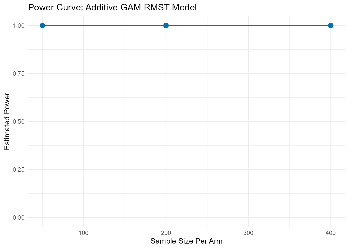

Sample Size Calculation

Scenario: We want to find the sample size needed to achieve 95% power for detecting an effect of pgr on recurrence-free survival.

ss_gam <- rmst.ss(
  Surv(rfstime, status) ~ s(pgr),
  data           = gbsg_prepared,
  arm            = "arm",
  target_power   = 0.95,
  L              = 182,
  n_sim          = 50,
  patience       = 5,
  parallel.cores = 1
)
--- Searching for Sample Size (Method: Additive GAM for RMST) ---
  N = 50/arm, Calculating Power... Power = 1

--- Simulation Summary ---


Table: Estimated Treatment Effect (RMST Difference)

|Statistic            |     Value|
|:--------------------|---------:|
|Mean RMST Difference | 90.790843|
|Mean Standard Error  |  0.193416|
|95% CI Lower         | 90.111979|
|95% CI Upper         | 91.469708|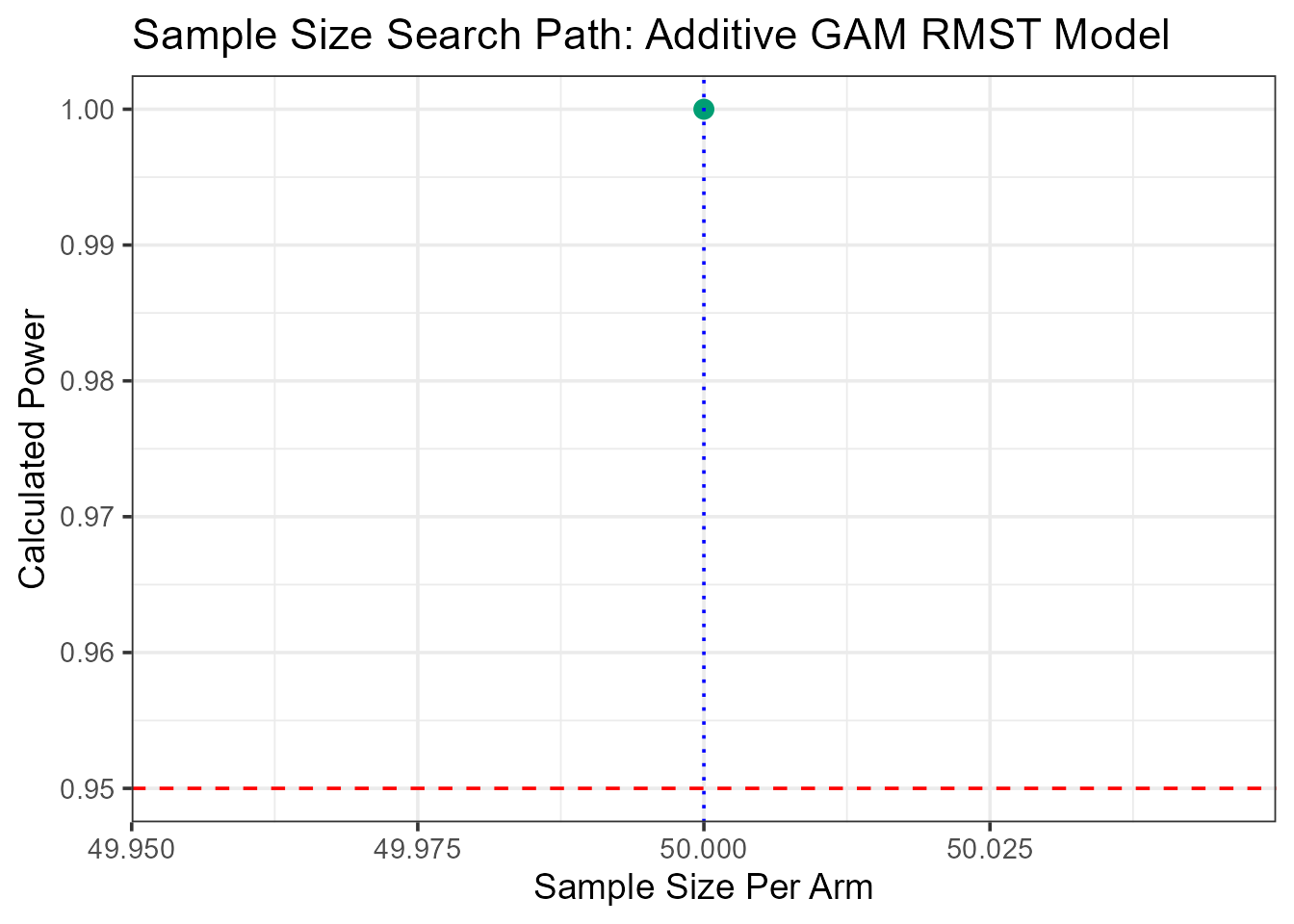

---

Covariate-Dependent Censoring Models

In many observational or longitudinal studies, the probability of being censored may depend on measured subject characteristics such as age, disease stage, or biomarker level, but not on the unobserved event time after conditioning on those covariates. This setting is referred to as covariate-dependent (or conditionally independent) censoring. Inverse-probability-of-censoring weighting (IPCW) can account for this dependence under the stated model and support valid estimation of the restricted mean survival time (RMST).

Theory and Model

We assume a single censoring mechanism described by a Cox proportional-hazards model for the censoring time: $$\text{Pr}(C \le t \mid X) = 1 - G(t \mid X), \qquad G(t \mid X) = \exp\{-\Lambda_C(t \mid X)\},$$ where $X$ denotes the observed covariates (e.g., age, sex, treatment arm). Each subject receives an inverse-probability weight $$W_i = \frac{1}{\widehat{G}(Y_i \mid X_i)}, \qquad Y_i = \min(T_i, L),$$ with $T_i$ the event time and $L$ the truncation horizon for RMST. Weights are stabilized and truncated to prevent numerical instability. The weighted regression $$E[Y_i \mid A_i, X_i] = \beta_0 + \beta_A A_i + X_i^\top\beta_X$$ is then fitted using weighted least squares. The variance of $\hat\beta_A$ is estimated with a sandwich-type estimator that treats the censoring model as known.

Power Calculation Formula

Analytic power is computed as $$\text{Power} = \Phi\!\left( \frac{|\hat\beta_A|}{\sigma_N} - z_{1-\alpha/2} \right), \qquad \sigma_N^2 = \frac{\widehat{\mathrm{Var}}(\hat\beta_A)}{N},$$ where $\widehat{\mathrm{Var}}(\hat\beta_A)$ is the asymptotic variance estimated from the reference data and $N$ is the total sample size. Because the same IPCW model is used for all subjects, no cause-specific components appear in the variance.

Analytical Methods

We demonstrate this approach using the mgus2 dataset, modeling censoring as a function of age and sex under a single censoring mechanism.

  id age sex dxyr  hgb creat mspike ptime pstat time death status arm
1  1  88   F 1981 13.1   1.3    0.5    30     0   30     1      0   0
2  2  78   F 1968 11.5   1.2    2.0    25     0   25     1      0   0
3  3  94   M 1980 10.5   1.5    2.6    46     0   46     1      0   1
4  4  68   M 1977 15.2   1.2    1.2    92     0   92     1      0   1
5  5  90   F 1973 10.7   0.8    1.0     8     0    8     1      0   0
6  6  90   M 1990 12.9   1.0    0.5     4     0    4     1      0   1

Power Calculation

Setting dep_cens = TRUE routes the call to the dependent-censoring adjusted estimator.

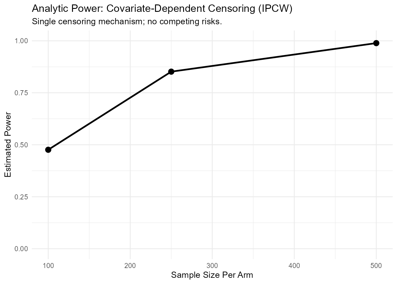
dc_power_results <- rmst.power(
  Surv(time, status) ~ age,
  data         = mgus_prepared,
  arm          = "arm",
  sample_sizes = c(100, 250, 500),
  L            = 120,
  dep_cens     = TRUE,
  alpha        = 0.05
)

Analytic Power Analysis under Covariate-Dependent Censoring

	Statistic	Value
arm	Assumed RMST Difference (from pilot)	-10.61349

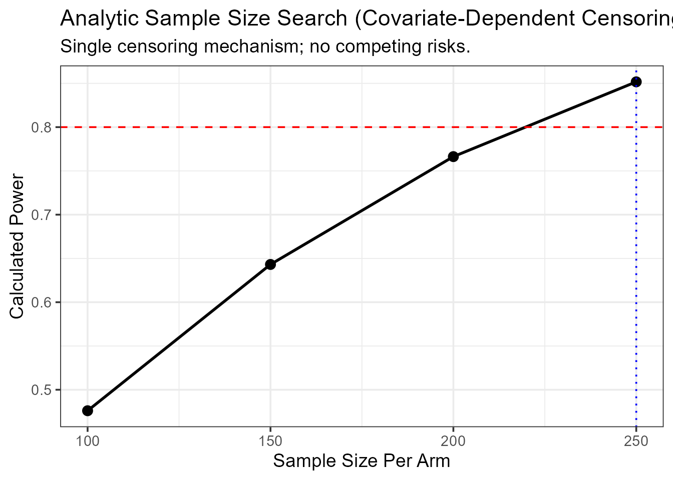
Sample-Size Calculation

We next estimate the per-arm sample size required to achieve 80% power at the same truncation time (10 years).

ss_dc_mgus <- rmst.ss(
  Surv(time, status) ~ age,
  data         = mgus_prepared,
  arm          = "arm",
  target_power = 0.80,
  L            = 120,
  dep_cens     = TRUE,
  alpha        = 0.05,
  n_start = 100, n_step = 50, max_n = 5000
)

--- Calculation Summary ---


Table: Required Sample Size

| Target_Power| Required_N_per_Arm|
|------------:|------------------:|
|          0.8|                250|

Estimated RMST Difference from Reference Data

	Statistic	Value
arm	Assumed RMST Difference (from pilot)	-10.61349

---

Interactive Shiny Application

RMSTpowerBoost also includes a Shiny web application for users who prefer a graphical interface.

Accessing the Application

There are two ways to access the application:

1. Live Web Version: Access the application directly in your browser without any installation.

   • Launch Web Application

2. Run Locally from the R Package: If you have installed the RMSTpowerBoost-Package, you can run the application on your own machine with the following command:

RMSTpowerBoost::run_app()

App Features

• Upload a reference dataset or generate data inside the app.
• Map input columns to the variables required for the analysis.
• Select the RMST model, calculation method, and analysis parameters.
• Review data summaries, Kaplan-Meier plots, result tables, and power curves.
• Export the analysis as PDF or HTML.

Conclusion

RMSTpowerBoost centers its interface on rmst.power() and rmst.ss() for RMST-based power and sample size calculations under linear, stratified, semiparametric, and covariate-dependent censoring models. Both functions use the familiar Surv(time, status) ~ covariates syntax, with model choice controlled by a small set of arguments (strata, strata_type, dep_cens, type).

In practice, these procedures depend on representative reference data because effect sizes and variance components are estimated from that dataset. Bootstrap-based methods can also require substantial computation.

Future development could extend simulation-based procedures for covariate-dependent censoring and add model diagnostic tools for assessing reference-data assumptions.

References

Andersen, Per K., Mette G. Hansen, and John P. Klein. 2004. “Regression Analysis of Restricted Mean Survival Time Based on Pseudo-Observations.” Lifetime Data Analysis 10 (4): 335–50. https://doi.org/10.1007/s10985-004-4771-0.

Parner, Erik T., and Per K. Andersen. 2010. “Regression Analysis of Censored Data Using Pseudo-Observations.” Stata Journal 10 (3): 408–22. https://doi.org/10.1177/1536867X1001000308.

Royston, Patrick, and Mahesh KB Parmar. 2013. “Restricted Mean Survival Time: An Alternative to the Hazard Ratio for the Design and Analysis of Randomized Trials with a Time-to-Event Outcome.” BMC Medical Research Methodology 13 (1): 1–13.

Tian, Lu, Lihui Zhao, and LJ Wei. 2014. “Predicting the Restricted Mean Event Time with the Subject’s Baseline Covariates in Survival Analysis.” Biostatistics 15 (2): 222–33.

Uno, Hajime, Brian Claggett, Lu Tian, et al. 2014. “Moving Beyond the Hazard Ratio in Quantifying the Between-Group Difference in Survival Analysis.” Journal of Clinical Oncology 32 (22): 2380.

Wang, Xin, and Douglas E Schaubel. 2018. “Modeling Restricted Mean Survival Time Under General Censoring Mechanisms.” Lifetime Data Analysis 24: 176–99.

Wang, Xin, Yingchao Zhong, Purna Mukhopadhyay, and Douglas E Schaubel. 2019. “Computationally Efficient Inference for Center Effects Based on Restricted Mean Survival Time.” Statistics in Medicine 38 (27): 5133–45.

Zhang, Yuan, and Douglas E Schaubel. 2024. “Semiparametric Additive Modeling of the Restricted Mean Survival Time.” Biometrical Journal 66 (6): e202200371.